Permutation tests in the Human Connectome Project

Posted on 07.December.2015 by A. M. Winkler

Permutation tests are known to be superior to parametric tests: they are based on only few assumptions, essentially that the data are exchangeable, and allow the correction for the multiplicity of tests and the use of various non-standard statistics. The exchangeability assumption allows data to be permuted whenever their joint distribution remains unaltered. Usually this means that each observation needs to be independent from the others.

In many studies, however, there are repeated measurements on the same subjects, which violates exchangeability: clearly, the various measurements obtained from a given subject are not independent from each other. In the Human Connectome Project (HCP) (Van Essen et al, 2012; 2013; see references at the end), subjects are sampled along with their siblings (most of them are twins), such that independence cannot be guaranteed either.

In Winkler et al. (2014), certain structured types of non-independence in brain imaging were addressed through the definition of exchangeability blocks (EBs). Observations within EB can be shuffled freely or, alternatively, the EBs themselves can be shuffled as a whole. This allows various designs that otherwise could not be assessed through permutations.

The same idea can be generalised for blocks that are nested within other blocks, in a multi-level fashion. In the paper Multi-level Block Permutation (Winkler et al., 2015) we presented a method that allows blocks to be shuffled a whole, and inside them, sub-blocks are further allowed to be shuffled, in a recursive process. The method is flexible enough to accommodate permutations, sign-flippings (sometimes also called “wild bootstrap”), and permutations together with sign-flippings.

In particular, this permutation scheme allows the data of the HCP to be analysed via permutations: subjects are allowed to be shuffled with their siblings while keeping the joint distribution intra-sibship maintained. Then each sibship is allowed to be shuffled with others of the same type.

In the paper we show that the error type I is controlled at the nominal level, and the power is just marginally smaller than that would be obtained by permuting freely if free permutation were allowed. The more complex the block structure, the larger the reductions in power, although with large sample sizes, the difference is barely noticeable.

Importantly, simply ignoring family structure in designs as this causes the error rates not to be controlled, with excess false positives, and invalid results. We show in the paper examples of false positives that can arise, even after correction for multiple testing, when testing associations between cortical thickness, cortical area, and measures of body size as height, weight, and body-mass index, all of them highly heritable. Such false positives can be avoided with permutation tests that respect the family structure.

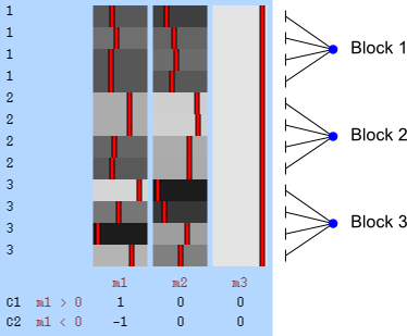
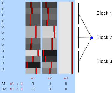
The figure at the top shows how the subjects of the HCP (terminal dots, shown in white colour) can be shuffled or not, while respecting the family structure. Blue dots indicate branches that can be permuted, whereas red dots indicate branches that cannot (see the main paper for details). This diagram includes 232 subjects of an early public release of HCP data. The tree on the left considers dizygotic twins as a category on their own, i.e., that cannot be shuffled with ordinary siblings, whereas the tree on the right considers dizygotic twins as ordinary siblings.

The first applied study using our strategy has just appeared. The method is implemented in the freely available package PALM — Permutation Analysis of Linear Models, and a set of practical steps to use it with actual HCP data is available here.

References

Van Essen DC, Ugurbil K, Auerbach E, Barch D, Behrens TE, Bucholz R, Chang A, Chen L, Corbetta M, Curtiss SW, Della Penna S, Feinberg D, Glasser MF, Harel N, Heath AC, Larson-Prior L, Marcus D, Michalareas G, Moeller S, Oostenveld R, Petersen SE, Prior F, Schlaggar BL, Smith SM, Snyder AZ, Xu J, Yacoub E; WU-Minn HCP Consortium. The Human Connectome Project: a data acquisition perspective. Neuroimage. 2012;62(4):2222-31.
Van Essen DC, Smith SM, Barch DM, Behrens TEJ, Yacoub E, Ugurbil K. The WU-Minn Human Connectome Project: An overview. Neuroimage. 2013;80:62-79.
Winkler AM, Ridgway GR, Webster MA, Smith SM, Nichols TE. Permutation inference for the general linear model. Neuroimage. 2014;92:381-97. (Open Access)
Winkler AM, Webster MA, Vidaurre D, Nichols TE, Smith SM. Multi-level block permutation. Neuroimage. 2015;123:253-68. (Open Access)

Another look into Pillai’s trace

Posted on 28.September.2015 by A. M. Winkler

In a previous post, all commonly used univariate and multivariate test statistics used with the general linear model (GLM) were presented. Here an alternative formulation for one of these statistics, the Pillai’s trace (Pillai, 1955, references at the end), commonly used in MANOVA and MANCOVA tests, is presented.

We begin with a multivariate general linear model expressed as:

$\mathbf{Y} = \mathbf{M} \boldsymbol{\psi} + \boldsymbol{\epsilon}$

where $\mathbf{Y}$ is the $N \times K$ full rank matrix of observed data, with $N$ observations of $K$ distinct (possibly non-independent) variables, $\mathbf{M}$ is the full-rank $N \times R$ design matrix that includes explanatory variables (i.e., effects of interest and possibly nuisance effects), $\boldsymbol{\psi}$ is the $R \times K$ vector of $R$ regression coefficients, and $\boldsymbol{\epsilon}$ is the $N \times K$ vector of random errors. Estimates for the regression coefficients can be computed as $\boldsymbol{\hat{\psi}} = \mathbf{M}^{+}\mathbf{Y}$ , where the superscript ( $^{+}$ ) denotes a pseudo-inverse.

The null hypothesis, and a simplification

One is generally interested in testing the null hypothesis that a contrast of regression coefficients is equal to zero, i.e., $\mathcal{H}_{0} : \mathbf{C}'\boldsymbol{\psi}\mathbf{D} = \boldsymbol{0}$ , where $\mathbf{C}$ is a $R \times S$ full-rank matrix of $S$ contrasts of coefficients on the regressors encoded in $\mathbf{X}$ , $1 \leqslant S \leqslant R$ and $\mathbf{D}$ is a $K \times Q$ full-rank matrix of $Q$ contrasts of coefficients on the dependent, response variables in $\mathbf{Y}$ , $1 \leqslant Q \leqslant K$ ; if $K=1$ or $Q=1$ , the model is univariate. Once the hypothesis has been established, $\mathbf{Y}$ can be equivalently redefined as $\mathbf{Y}\mathbf{D}$ , such that the contrast $\mathbf{D}$ can be omitted for simplicity, and the null hypothesis stated as $\mathcal{H}_{0} : \mathbf{C}'\boldsymbol{\psi} = \boldsymbol{0}$ .

Model partitioning

It is useful to consider a transformation of the model into a partitioned one:

$\mathbf{Y} = \mathbf{X}\boldsymbol{\beta} + \mathbf{Z}\boldsymbol{\gamma} + \boldsymbol{\epsilon}$

where $\mathbf{X}$ is the matrix with regressors of interest, $\mathbf{Z}$ is the matrix with nuisance regressors, and $\boldsymbol{\beta}$ and $\boldsymbol{\gamma}$ are respectively the vectors of regression coefficients. From this model we can also define the projection (hat) matrices $\mathbf{H}_{\mathbf{X}}=\mathbf{X}\mathbf{X}^{+}$ and $\mathbf{H}_{\mathbf{Z}}=\mathbf{Z}\mathbf{Z}^{+}$ due to tue regressors of interest and nuisance, respectively, and the residual-forming matrices $\mathbf{R}_{\mathbf{X}}=\mathbf{I}-\mathbf{H}_{\mathbf{X}}$ and $\mathbf{R}_{\mathbf{Z}}=\mathbf{I}-\mathbf{H}_{\mathbf{Z}}$ .

Such partitioning is not unique, and schemes can be as simple as separating apart the columns of $\mathbf{M}$ as $\left[ \mathbf{X} \; \mathbf{Z} \right]$ , with $\boldsymbol{\psi} = \left[ \boldsymbol{\beta}' \; \boldsymbol{\gamma}' \right]'$ . More involved strategies can, however, be devised to obtain some practical benefits. One such partitioning is to define $\mathbf{X} = \mathbf{M} \mathbf{Q} \mathbf{C} \left(\mathbf{C}'\mathbf{Q}\mathbf{C}\right)^{-1}$ and
$\mathbf{Z} = \mathbf{M} \mathbf{Q} \mathbf{C}_v \left(\mathbf{C}_v'\mathbf{Q}\mathbf{C}_v\right)^{-1}$ , where $\mathbf{Q}=(\mathbf{M}'\mathbf{M})^{-1}$ , $\mathbf{C}_v=\mathbf{C}_u-\mathbf{C}(\mathbf{C}'\mathbf{Q}\mathbf{C})^{-1}\mathbf{C}'\mathbf{Q}\mathbf{C}_u$ , and $\mathbf{C}_u$ has $r-\mathsf{rank}\left(\mathbf{C}\right)$ columns that span the null space of $\mathbf{C}$ , such that $[\mathbf{C} \; \mathbf{C}_u]$ is a $r \times r$ invertible, full-rank matrix (Smith et al, 2007). This partitioning has a number of features: $\boldsymbol{\hat{\beta}} = \mathbf{C}'\boldsymbol{\hat{\psi}}$ , $\widehat{\mathsf{Cov}}(\boldsymbol{\hat{\beta}}) = \mathbf{C}'\widehat{\mathsf{Cov}}(\boldsymbol{\hat{\psi}})\mathbf{C}$ , i.e., estimates and variances of $\boldsymbol{\beta}$ for inference on the partitioned model correspond exactly to the same inference on the original model, $\mathbf{X}$ is orthogonal to $\mathbf{Z}$ , and $\mathsf{span}(\mathbf{X}) \cup \mathsf{span}(\mathbf{Z}) = \mathsf{span}(\mathbf{M})$ , i.e., the partitioned model spans the same space as the original.

Another partitioning scheme, derived by Ridgway (2009), defines $\mathbf{X}=\mathbf{M}(\mathbf{C}^+)'$ and $\mathbf{Z}=\mathbf{M}-\mathbf{M}\mathbf{C}\mathbf{C}^{+}$ . As with the previous strategy, the parameters of interest in the partitioned model are equal to the contrast of the original parameters. A full column rank nuisance partition can be obtained from the singular value decomposition (SVD) of $\mathbf{Z}$ , which will also provide orthonormal columns for the nuisance partition. Orthogonality between regressors of interest and nuisance can be obtained by redefining the regressors of interest as $\mathbf{R}_{\mathbf{Z}}\mathbf{X}$ .

The usual multivariate statistics

For the multivariate statistics, define generically:

$\mathbf{H}=(\mathbf{C}'\boldsymbol{\hat{\psi}}\mathbf{D})' \left(\mathbf{C}'(\mathbf{M}'\mathbf{M})^{-1}\mathbf{C} \right)^{-1} (\mathbf{C}'\boldsymbol{\hat{\psi}}\mathbf{D})$

as the sums of products explained by the model (hypothesis) and:

$\mathbf{E} = (\boldsymbol{\hat{\epsilon}}\mathbf{D})'(\boldsymbol{\hat{\epsilon}}\mathbf{D})$

as the sums of the products of the residuals, i.e., that remain unexplained. With the simplification to the original model that redefined $\mathbf{Y}$ as $\mathbf{Y}\mathbf{D}$ , the $\mathbf{D}$ can be dropped, so that we have $\mathbf{H}=(\mathbf{C}'\boldsymbol{\hat{\psi}})' \left(\mathbf{C}'(\mathbf{M}'\mathbf{M})^{-1}\mathbf{C} \right)^{-1} (\mathbf{C}'\boldsymbol{\hat{\psi}})$ and $\mathbf{E} = \boldsymbol{\hat{\epsilon}}'\boldsymbol{\hat{\epsilon}}$ . The various well-known multivariate statistics (see this earlier blog entry) can be written as a function of $\mathbf{H}$ and $\mathbf{E}$ . Pillai’s trace is:

$T=\mathsf{trace}\left(\mathbf{H}(\mathbf{H}+\mathbf{E})^{-1}\right)$

More simplifications

With the partitioning, other simplifications are possible:

$\mathbf{H}=\boldsymbol{\hat{\beta}}' (\mathbf{X}'\mathbf{X})\boldsymbol{\hat{\beta}} = ( \mathbf{X}\boldsymbol{\hat{\beta}})'(\mathbf{X}\boldsymbol{\hat{\beta}})$

Recalling that $\mathbf{X}'\mathbf{Z}=\mathbf{0}$ , and defining $\tilde{\mathbf{Y}}=\mathbf{R}_{\mathbf{Z}}\mathbf{Y}$ , we have:

$\mathbf{H} = (\mathbf{H}_{\mathbf{X}}\tilde{\mathbf{Y}})'(\mathbf{H}_{\mathbf{X}}\tilde{\mathbf{Y}}) = \tilde{\mathbf{Y}}'\mathbf{H}_{\mathbf{X}}\tilde{\mathbf{Y}}$

The unexplained sums of products can be written in a similar manner:

$\mathbf{E} = (\mathbf{R}_{\mathbf{X}}\tilde{\mathbf{Y}})'(\mathbf{R}_{\mathbf{X}}\tilde{\mathbf{Y}}) = \tilde{\mathbf{Y}}'\mathbf{R}_{\mathbf{X}}\tilde{\mathbf{Y}}$

The term $\mathbf{H}+\mathbf{E}$ in the Pillai’s trace can therefore be rewritten as:

$\mathbf{H}+\mathbf{E}= \tilde{\mathbf{Y}}'(\mathbf{H}_{\mathbf{X}} + \mathbf{R}_{\mathbf{X}})\tilde{\mathbf{Y}} = \tilde{\mathbf{Y}}'\tilde{\mathbf{Y}}$

Using the property that the trace of a product is invariant to a circular permutation of the factors, Pillai’s statistic can then be written as:

$\begin{array}{ccl} T&=&\mathsf{trace}\left(\tilde{\mathbf{Y}}'\mathbf{H}_{\mathbf{X}}\tilde{\mathbf{Y}}\left(\tilde{\mathbf{Y}}'\tilde{\mathbf{Y}}\right)^{+}\right)\\ {}&=&\mathsf{trace}\left(\mathbf{H}_{\mathbf{X}}\tilde{\mathbf{Y}}\left(\tilde{\mathbf{Y}}'\tilde{\mathbf{Y}}\right)^{+}\tilde{\mathbf{Y}}'\right)\\ {}&=&\mathsf{trace}\left(\mathbf{H}_{\mathbf{X}}\tilde{\mathbf{Y}}\tilde{\mathbf{Y}}^{+}\right)\\ \end{array}$

The final, alternative form

Using sigular value decomposition we have $\tilde{\mathbf{Y}} = \mathbf{U}\mathbf{S}\mathbf{V}'$ and $\tilde{\mathbf{Y}}^{+} = \mathbf{V}\mathbf{S}^{+}\mathbf{U}'$ , where $\mathbf{U}$ contains only the columns that correspond to non-zero eigenvalues. Thus, the above can be rewritten as:

$\begin{array}{ccl} T&=&\mathsf{trace}\left(\mathbf{H}_{\mathbf{X}} \mathbf{U}\mathbf{S}\mathbf{V}' \mathbf{V}\mathbf{S}^{+}\mathbf{U}' \right)\\ {}&=&\mathsf{trace}\left(\mathbf{H}_{\mathbf{X}} \mathbf{U}\mathbf{U}' \right)\\ \end{array}$

The SVD transformation is useful for languages or libraries that offer a fast implementation. Otherwise, using a pseudoinverse yields the same result, perhaps only slightly slower. In this case, $T=\mathsf{trace}\left(\mathbf{H}_{\mathbf{X}}\tilde{\mathbf{Y}}\tilde{\mathbf{Y}}^{+}\right)$ .

Importance

If we define $\mathbf{A}\equiv\mathbf{H}_{\mathbf{X}}$ and $\mathbf{W}\equiv\mathbf{U}\mathbf{U}'$ (or $\mathbf{W}\equiv\tilde{\mathbf{Y}}\tilde{\mathbf{Y}}^{+}$ ), then $T=\mathsf{trace}\left(\mathbf{A}\mathbf{W}\right)$ . The first three moments of the permutation distribution of statistics that can be written in this form can be computed analytically once $\mathbf{A}$ and $\mathbf{W}$ are known. With the first three moments, a gamma distribution (Pearson type III) can be fit, thus allowing p-values to be computed without resorting to the usual beta approximation to Pillai’s trace, nor using permutations, yet with results that are not based on the assumption of normality (Mardia, 1971; Kazi-Aoual, 1995; Minas and Montana, 2014).

Availability

This simplification is available in PALM, for use with imaging and non-imaging data, using Pillai’s trace itself, or a modification that allows inference on univariate statistics. As of today, this option is not yet documented, but should become openly available soon.

References

Kazi-Aoual F, Hitier S, Sabatier R, Lebreton J-D. Refined approximations to permutation tests for multivariate inference. Comput Stat Data Anal. 1995;20(94):643–56.
Mardia KV. The Effect of Nonnormality on some multivariate tests and robustness to nonnormality in the linear model. Biometrika. 1971;58(1):105–21.
Minas C, Montana G. Distance-based analysis of variance: Approximate inference. Stat Anal Data Min. 2014;7(6):450–70.
Pillai KCS. Some New test criteria in multivariate analysis. Ann Math Stat. 1955;26(1):117–21.
Ridgway GR. Statistical analysis for longitudinal MR imaging of dementia. PhD Thesis. University College London, 2009.
Smith SM, Jenkinson M, Beckmann CF, Miller K, Woolrich M. Meaningful design and contrast estimability in FMRI. Neuroimage. 2007;34(1):127–36.
Winkler AM, Ridgway GR, Webster MA, Smith SM, Nichols TE. Permutation inference for the general linear model. Neuroimage. 2014;92:381–97.

Update: 20.Jan.2016: A slight simplification was applied to the formulas above so as to make them more elegant and remove some redundancy. The result is the same.

The lady tasting tea experiment

Posted on 23.August.2015 by A. M. Winkler

Can you tell?

The now famous story is that in an otherwise unremarkable summer afternoon in Cambridge in the 1920’s, a group of friends eventually discussed about the claims made by one of the presents about her abilities on discriminating whether milk was poured first or last when preparing a cup of tea with milk. One of the presents was Ronald Fisher, and the story, along with a detailed description of how to conduct a simple experiment to test the claimed ability, and how to obtain an exact solution, was presented at length in the Chapter 2 of his book The Design of Experiments, a few lines of which are quoted below:

A lady declares that by tasting a cup of tea made with milk she can discriminate whether the milk or the tea infusion was first added to the cup. We will consider the problem of designing an experiment by means of which this assertion can be tested. […] [It] consists in mixing eight cups of tea, four in one way and four in the other, and presenting them to the subject for judgment in a random order. The subject has been told in advance of that the test will consist, namely, that she will be asked to taste eight cups, that these shall be four of each kind […]. — Fisher, 1935.

There are $\frac{8!}{4!4!}=70$ distinct possible orderings of these cups, and by telling the subject in advance that there are four cups of each type, this guarantees that the answer will include four of each.

The lady in question eventually answered correctly six out of the eight trials. The results can be assembled in a 2 by 2 contingency table:

		True order:		Total (margin)
		Tea first	Milk first	Total (margin)
Lady’s Guesses:	Tea first	$a=3$	$b=1$	$a+b=4$
Lady’s Guesses:	Milk first	$c=1$	$d=3$	$c+d=4$
Total (margin)		$a+c=4$	$b+d=4$	$n=8$

With these results, what should be concluded about the ability of the lady in discriminating whether milk or tea was poured first? It is not possible to prove that she would never be wrong, because if a sufficiently large number of cups of tea were offered, a single failure would disprove such hypothesis. However, a test that she is never right can be disproven, with a certain margin of uncertainty, given the number of cups offered.

Solution using Fisher’s exact method

Fisher presented an exact solution for this experiment. It is exact in the sense that it allows an exact probability to be assigned to each of the possible outcomes. The probability can be calculated as:

$P_{\text{Fisher}} = \dfrac{(a+b)!(c+d)!(a+c)!(b+d)!}{n!a!b!c!d!}$

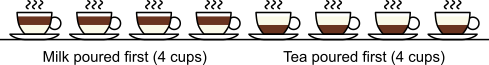
For the particular configuration of the contingency table above, the probability is $\frac{16}{70} = 0.22857$ . This is not the final result, though: what matters to disprove the hypothesis that she is not able to discriminate is how likely it would be for her to find a result at least as extreme as the one observed. In this case, there is one case that is more extreme, which would be the one in which she would have made correct guesses for all the 8 cups, in which case the values in the contingency table above would have been $a = 4$ , $b = 0$ , $c = 0$ , and $d = 4$ , with a probability computed with the same formula as $\frac{1}{70} = 0.01429$ . Adding these two probabilities together yield $\frac{16+1}{70}=0.24286$ .

Thus, if the lady is not able to discriminate whether tea or milk was poured first, the chance of observing a result at least as favourable towards her claim would be 0.24286, i.e., about 24%.

If from the outset we were willing to consider a significance level 0.05 (5%) as an informal rule to disprove the null hypothesis, we would have considered the p-value = 0.24286 as non-significant. This p-value is exact, a point that will become more clear below, in the section about permutation tests.

Using the hypergeometric distribution directly

The above process can become laborious for experiments with larger number of trials. An alternative, but equivalent solution, is to appeal directly to the hypergeometric distribution. The probability mass function (pmf) of this distribution can be written as a function the parameters of the contingency table as:

$P(X=a) = \dfrac{\binom{a+b}{a}\binom{c+d}{c}}{\binom{n}{a+c}}$

The pmf is equivalent to Fisher’s exact formula to compute the probability of a particular configuration. The cumulative density function, which is conditional on the margins being fixed, is:

$P(X \geqslant a) = \sum_{j=a}^{J}\dfrac{\binom{a+b}{j}\binom{c+d}{a+c-j}}{\binom{n}{a+c}} = \sum_{j=a}^{J}\dfrac{(a+b)!(c+d)!(a+c)!(b+d)!}{n!j!(a+b-j)!(a+c-j)!(d-a+j)!}$

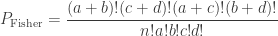
where $J=\min(a+c,a+b)$ . Computing from the above (details omitted), yield the same value as using Fisher’s presentation, that is, the p-value is (exactly) 0.24286.

Solution using Pearson’s $\chi^2$ method

Much earlier than the tea situation described above, Karl Pearson had already considered the problem of inference in contingency tables, having proposed a test based on a $\chi^2$ statistic.

$\chi^2 = \sum_{i=1}^{R}\sum_{j=1}^{C}\dfrac{(O_{ij}-E_{ij})^2}{E_{ij}}$

where $O_{ij}$ is the observed value for the element in the position $(i,j)$ in the table, $R$ and $C$ are respectively the number of rows and columns, and $E_{ij}$ is the expected value for these elements if the null hypothesis is true. The values $E_{ij}$ can be computed as the product of the marginals for row $i$ and column $j$ , divided by the overall number of observations $n$ . A simpler, equivalent formula is given by:

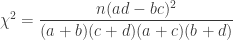
$\chi^2 = \dfrac{n(ad - bc)^2}{(a+b)(c+d)(a+c)(b+d)}$

A p-value can be computed from the $\chi^2$ distribution with degrees of freedom $\nu=(R-1)(C-1)$ .

Under the null, we can expect a value equal to 2 in each of the 2 cells, that is, the lady would for each cup have a 50:50 chance of answering correctly. For the original tea tasting experiment, Pearson’s method give quite inaccurate results: $\chi^2=2$ , which corresponds to a p-value of 0.07865. However, it is well known that this method is inaccurate if cells in the table have too small quantities, usually below 5 or 6.

Improvement using Yates’ continuity correction

To solve the above well-known issue with small quantities, Yates (1934) proposed a correction, such that the test statistic becomes:

$\chi^2 = \sum_{i,j}\dfrac{\left(|O_{ij}-E_{ij}|-\frac{1}{2}\right)^2}{E_{ij}}$

Applying this correction to the original tea experiment gives $\chi^2=0.5$ , and a p-value of 0.23975, which is very similar to the one given by the Fisher method. Note again that this approach, like the $\chi^2$ test, predates Fisher’s exact test.

Equivalence of Fisher’s exact test and permutation tests

The method proposed by Fisher corresponds to a permutation test. Let $\mathbf{x}$ be a column vector containing binary indicators for whether milk was truly poured first. Let $\mathbf{y}$ be a column vector containing binary indicators for whether the lady answered that milk was poured first. The general linear model (GLM) can be used as usual, such that $\mathbf{y}=\mathbf{x}\beta + \boldsymbol{\epsilon}$ , where $\beta$ is a regression coefficient, and $\boldsymbol{\epsilon}$ are the residuals.

Under the null hypothesis that the lady cannot discriminate, the binary values in $\mathbf{y}$ can be permuted randomly. There are $\binom{8}{4}=70$ possible unique rearrangements. Out of these, in 17, there are 6 or more (out of 8) correct answers matching the values in $\mathbf{x}$ , which gives a p-value 17/70 = 0.24286.

Note that the strategy using the GLM can be used even if both variables $\mathbf{x}$ and $\mathbf{y}$ are binary, as in the example of the tea tasting, even if the residuals are not normally distributed (permutation tests do not depend on distributional assumptions), and even considering that values in $\beta$ can lead to non-sensical predictions in $\mathbf{y}$ , as prediction is not the objective of this analysis.

Why not a binomial test?

The binomial test could be considered if the lady did not know in advance that there were 4 cups of each mixture order. Since she knew (so the two margins of the table are fixed), each cup was not independent from each other, and her possible answers had to be constrained by answers previously given. The binomial test assumes independence, thus, is not an option for this analysis.

Relevance

Using this simple experiment, Fisher established most of the fundamental principles for hypothesis testing, which contributed to major advances across biological and physical sciences. A careful read of the original text shows a precise use of terms, in a concise and unambiguous presentation, in contrast with many later and more verbose textbooks that eventually hid from readers most of the fundamental principles.

References

Fisher, R. A. The Design of Experiments. Oliver and Boyd, Edinburgh, 1935.
Pearson K. X. On the criterion that a given system of deviations from the probable in the case of a correlated system of variables is such that it can be reasonably supposed to have arisen from random sampling. Philos Mag Ser 5. 1900 Jul;50(302):157–75.
Yates F. Contingency Tables Involving Small Numbers and the Chi^2 test. Suppl to J R Stat Soc. 1934;1(2):217–35.

The photograph at the top (tea with milk) is in public domain.

Variance components in genetic analyses

Posted on 02.August.2015 by A. M. Winkler

Pedigree-based analyses allow investigation of genetic and environmental influences on anatomy, physiology, and behaviour.

Methods based on components of variance have been used extensively to assess genetic influences and identify loci associated with various traits quantifying aspects of anatomy, physiology, and behaviour, in both normal and pathological conditions. In an earlier post, indices of genetic resemblance between relatives were presented, and in the last post, the kinship matrix was defined. In this post, these topics are used to present a basic model that allows partitioning of the phenotypic variance into sources of variation that can be ascribed to genetic, environmental, and other factors.

A simple model

Consider the model:

$\mathbf{Y} = \mathbf{X}\mathbf{B} + \boldsymbol{\Upsilon}$

where, for $S$ subjects, $T$ traits, $P$ covariates and $K$ variance components, $\mathbf{Y}_{S \times T}$ are the observed trait values for each subject, $\mathbf{X}_{S \times P}$ is a matrix of covariates, $\mathbf{B}_{P \times T}$ is a matrix of unknown covariates’ weights, and $\boldsymbol{\Upsilon}_{S \times T}$ are the residuals after the covariates have been taken into account.

The elements of each column $t$ of $\boldsymbol{\Upsilon}$ are assumed to follow a multivariate normal distribution $\mathcal{N}\left(0;\mathbf{S}\right)$ , where $\mathbf{S}$ is the between-subject covariance matrix. The elements of each row $s$ of $\boldsymbol{\Upsilon}$ are assumed to follow a normal distribution $\mathcal{N}\left(0;\mathbf{R}\right)$ , where $\mathbf{R}$ is the between-trait covariance matrix. Both $\mathbf{R}$ and $\mathbf{S}$ are seen as the sum of $K$ variance components, i.e. $\mathbf{R} = \sum_{k} \mathbf{R}_{k}$ and $\mathbf{S} = \sum_{k} \mathbf{S}_{k}$ . For a discussion on these equalities, see Eisenhart (1947) [see references at the end].

An equivalent model

The same model can be written in an alternative way. Let $\mathbf{y}_{S \cdot T \times 1}$ be the stacked vector of traits, $\mathbf{\tilde{X}}_{S \cdot T \times P \cdot T} = \mathbf{X} \otimes \mathbf{I}_{T \times T}$ is the matrix of covariates, $\boldsymbol{\beta}_{P \cdot T \times 1}$ the vector with the covariates’ weights, $\boldsymbol{\upsilon}_{S \cdot T \times 1}$ the residuals after the covariates have been taken into account, and $\otimes$ represent the Kronecker product. The model can then be written as:

$\mathbf{y} = \mathbf{\tilde{X}}\boldsymbol{\beta} + \boldsymbol{\upsilon}$

The stacked residuals $\boldsymbol{\upsilon}$ is assumed to follow a multivariate normal distribution $\mathcal{N}\left(0;\boldsymbol{\Omega}\right)$ , where $\boldsymbol{\Omega}$ can be seen as the sum of $K$ variance components:

$\boldsymbol{\Omega} = \sum_{k} \mathbf{R}_k \otimes \mathbf{S}_k$

The $\boldsymbol{\Omega}$ here is the same as in Almasy and Blangero (1998). $\mathbf{S}_k$ can be modelled as correlation matrices. The associated scalars are absorbed into the (to be estimated) $\mathbf{R}_k$ . $\mathbf{R}$ is the phenotypic covariance matrix between the residuals of the traits:

$\mathbf{R} = \left[ \begin{array}{ccc} \mathsf{Var}(\upsilon_1) & \cdots & \mathsf{Cov}(\upsilon_1,\upsilon_T) \\ \vdots & \ddots & \vdots \\ \mathsf{Cov}(\upsilon_T,\upsilon_1) & \cdots & \mathsf{Var}(\upsilon_T) \end{array}\right]$

whereas each $\mathbf{R}_k$ are the share of these covariances attributable to the $k$ -th component:

$\mathbf{R}_k = \left[ \begin{array}{ccccc} \mathsf{Var}_k(\upsilon_1) & \cdots & \mathsf{Cov}_k(\upsilon_1,\upsilon_T) \\ \vdots & \ddots & \vdots \\ \mathsf{Cov}_k(\upsilon_T,\upsilon_1) & \cdots & \mathsf{Var}_k(\upsilon_T) \end{array}\right]$

$\mathbf{R}$ can be converted to a between-trait phenotypic correlation matrix $\mathbf{\mathring{R}}$ as:

$\mathbf{\mathring{R}} = \left[ \begin{array}{ccc} \frac{\mathsf{Var}(\upsilon_1)}{\mathsf{Var}(\upsilon_1)} & \cdots & \frac{\mathsf{Cov}(\upsilon_1,\upsilon_T)}{\left(\mathsf{Var}(\upsilon_1)\mathsf{Var}(\upsilon_T)\right)^{1/2}} \\ \vdots & \ddots & \vdots \\ \frac{\mathsf{Cov}(\upsilon_1,\upsilon_T)}{\left(\mathsf{Var}(\upsilon_1)\mathsf{Var}(\upsilon_T)\right)^{1/2}} & \cdots & \frac{\mathsf{Var}(\upsilon_T)}{\mathsf{Var}(\upsilon_T)} \end{array}\right]$

The above phenotypic correlation matrix has unit diagonal and can still be fractioned into their $K$ components:

$\mathbf{\mathring{R}}_k = \left[ \begin{array}{ccc} \frac{\mathsf{Var}_k(\upsilon_1)}{\mathsf{Var}(\upsilon_1)} & \cdots & \frac{\mathsf{Cov}_k(\upsilon_1,\upsilon_T)}{\left(\mathsf{Var}(\upsilon_1)\mathsf{Var}(\upsilon_T)\right)^{1/2}} \\ \vdots & \ddots & \vdots \\ \frac{\mathsf{Cov}_k(\upsilon_T,\upsilon_1)}{\left(\mathsf{Var}(\upsilon_T)\mathsf{Var}(\upsilon_1)\right)^{1/2}} & \cdots & \frac{\mathsf{Var}_k(\upsilon_T)}{\mathsf{Var}(\upsilon_T)} \end{array}\right]$

The relationship $\mathbf{\mathring{R}} = \sum_k \mathbf{\mathring{R}}_k$ holds. The diagonal elements of $\mathbf{\mathring{R}}_k$ may receive particular names, e.g., heritability, environmentability, dominance effects, shared enviromental effects, etc., depending on what is modelled in the corresponding $\mathbf{S}_k$ . However, the off-diagonal elements of $\mathbf{\mathring{R}}_k$ are not the $\rho_k$ that correspond, e.g. to the genetic or environmental correlation. These off-diagonal elements are instead the signed $\text{\textsc{erv}}$ when $\mathbf{S}_k=2\cdot\boldsymbol{\Phi}$ , or their $\text{\textsc{erv}}_k$ -equivalent for other variance components (see below). In this particular case, they can also be called “bivariate heritabilities” (Falconer and MacKay, 1996). A matrix $\mathbf{\breve{R}}_k$ that contains these correlations $\rho_k$ , which are the fraction of the variance attributable to the $k$ -th component that is shared between pairs of traits is given by:

$\mathbf{\breve{R}}_k = \left[ \begin{array}{ccc} \frac{\mathsf{Var}_k(\upsilon_1)}{\mathsf{Var}_k(\upsilon_1)} & \cdots & \frac{\mathsf{Cov}_k(\upsilon_1,\upsilon_T)}{\left(\mathsf{Var}_k(\upsilon_1)\mathsf{Var}_k(\upsilon_T)\right)^{1/2}} \\ \vdots & \ddots & \vdots \\ \frac{\mathsf{Cov}_k(\upsilon_T,\upsilon_1)}{\left(\mathsf{Var}_k(\upsilon_T)\mathsf{Var}_k(\upsilon_1)\right)^{1/2}} & \cdots & \frac{\mathsf{Var}_k(\upsilon_T)}{\mathsf{Var}_k(\upsilon_T)} \end{array}\right]$

As for the phenotypic correlation matrix, each $\mathbf{\breve{R}}_k$ has unit diagonal.

The most common case

A particular case is when $\mathbf{S}_1 = 2\cdot\boldsymbol{\Phi}$ , the coefficient of familial relationship between subjects, and $\mathbf{S}_2 = \mathbf{I}_{S \times S}$ . In this case, the $T$ diagonal elements of $\mathbf{\mathring{R}}_1$ represent the heritability ( $h_t^2$ ) for each trait $t$ . The diagonal of $\mathbf{\mathring{R}}_2$ contains $1-h_t^2$ , the environmentability. The off-diagonal elements of $\mathbf{\mathring{R}}_1$ contain the signed $\text{\textsc{erv}}$ (see below). The genetic correlations, $\rho_g$ are the off-diagonal elements of $\mathbf{\breve{R}}_1$ , whereas the off-diagonal elements of $\mathbf{\breve{R}}_2$ are $\rho_e$ , the environmental correlations between traits. In this particular case, the components of $\mathbf{R}$ , i.e., $\mathbf{R}_k$ are equivalent to $\mathbf{G}$ and $\mathbf{E}$ covariance matrices as in Almasy et al (1997).

Relationship with the ERV

To see how the off-diagonal elements of $\mathbf{\mathring{R}}_k$ are the signed Endophenotypic Ranking Values for each of the $k$ -th variance component, $\text{\textsc{erv}}_k$ (Glahn et al, 2011), note that for a pair of traits $i$ and $j$ :

$\mathring{R}_{kij} = \frac{\mathsf{Cov}_k(\upsilon_i,\upsilon_j)}{\left(\mathsf{Var}(\upsilon_i)\mathsf{Var}(\upsilon_j)\right)^{1/2}}$

Multiplying both numerator and denominator by $\left(\mathsf{Var}_k(\upsilon_i)\mathsf{Var}_k(\upsilon_j)\right)^{1/2}$ and rearranging the terms gives:

$\mathring{R}_{kij} = \frac{\mathsf{Cov}_k(\upsilon_i,\upsilon_j)}{\left(\mathsf{Var}_k(\upsilon_i)\mathsf{Var}_k(\upsilon_j)\right)^{1/2}} \left(\frac{\mathsf{Var}_k(\upsilon_i)}{\mathsf{Var}(\upsilon_i)}\frac{\mathsf{Var}_k(\upsilon_j)}{\mathsf{Var}(\upsilon_j)}\right)^{1/2}$

When $\mathbf{S}_k = 2\cdot\boldsymbol{\Phi}$ , the above reduces to $\mathring{R}_{kij} = \rho_k \sqrt{h^2_i h^2_j}$ , which is the signed version of $\text{\textsc{erv}}=\left|\rho_g\sqrt{h_i^2h_j^2}\right|$ when $k$ is the genetic component.

Positive-definiteness

$\mathbf{R}$ and $\mathbf{R}_k$ are covariance matrices and so, are positive-definite, whereas the correlation matrices $\mathbf{\mathring{R}}$ , $\mathbf{\mathring{R}}_k$ and $\mathbf{\breve{R}}_k$ are positive-semidefinite. A hybrid matrix that does not have to be positive-definite or semidefinite is:

$\mathbf{\check{R}}_k = \mathbf{I} \odot \mathbf{\mathring{R}}_k + \left(\mathbf{J}-\mathbf{I}\right) \odot \mathbf{\breve{R}}_k$

where $\mathbf{J}$ is a matrix of ones, $\mathbf{I}$ is the identity, both of size $T \times T$ , and $\odot$ is the Hadamard product. An example of such matrix of practical use is to show concisely the heritabilities for each trait in the diagonal and the genetic correlations in the off-diagonal.

Cauchy-Schwarz

Algorithmic advantages can be obtained from the positive-definiteness of $\mathbf{\mathring{R}}_k$ . The Cauchy–Schwarz theorem (Cauchy, 1821; Schwarz, 1888) states that:

$\mathring{R}_{kij} \leqslant \sqrt{\mathring{R}_{kii}\mathring{R}_{kjj}}$

Hence, the bounds for the off-diagonal elements can be known from the diagonal elements, which, by their turn, are estimated in a simpler, univariate model.

The Cauchy-Schwarz inequality imposes limits on the off-diagonal values of the matrix that contains the genetic covariances (or bivariate heritabilities).

Parameter estimation

Under the multivariate normal assumption, the parameters can be estimated maximising the following loglikelihood function:

$\mathcal{L}\left(\mathbf{R}_k,\boldsymbol{\beta}\Big|\mathbf{y},\mathbf{\tilde{X}}\right) = -\frac{1}{2} \left(N \ln 2\pi + \ln \left|\boldsymbol{\Omega}\right| + \left(\mathbf{y}-\mathbf{\tilde{X}}\boldsymbol{\beta}\right)'\boldsymbol{\Omega}\left(\mathbf{y}-\mathbf{\tilde{X}}\boldsymbol{\beta}\right)\right)$

where $N=S \cdot T$ is the number of observations on the stacked vector $\mathbf{y}$ . Unbiased estimates for $\boldsymbol{\beta}$ , although inefficient and inappropriate for hypothesis testing, can be obtained with ordinary least squares (OLS).

Parametric inference

Hypothesis testing can be performed with the likelihood ratio test (LRT), i.e., the test statistic is produced by subtracting from the loglikelihood of the model in which all the parameters are free to vary ( $\mathcal{L}_1$ ), the loglikelihood of a model in which the parameters being tested are constrained to zero, the null model ( $\mathcal{L}_0$ ). The statistic is given by $\lambda = 2\left(\mathcal{L}_1-\mathcal{L}_0\right)$ (Wilks, 1938), which here is asymptotically distributed as a 50:50 mixture of a $\chi^2_0$ and $\chi^2_{\text{df}}$ distributions, where df is the number of parameters being tested and free to vary in the unconstrained model (Self and Liang, 1987). From this distribution the p-values can be obtained.

References

Almasy L, Blangero J. Multipoint quantitative-trait linkage analysis in general pedigrees. Am J Hum Genet. 1998 May;62(5):1198–211.
Almasy L, Dyer TD, Blangero J. Bivariate quantitative trait linkage analysis: pleiotropy versus co-incident linkages. Genet Epidemiol. 1997 Jan;14(6):953–8.
Cauchy, A-L. Œuvres Completes D’Augustin Cauchy (published in 1882). Vol. XV. Gauthier-Villars et Fils, Paris, 1821.
Eisenhart C. The assumptions underlying the analysis of variance. Biometrics. 1947;3(1):1–21.
Falconer DS, Mackay TFC. Introduction to Quantitative Genetics. Addison Wesley Longman, Harlow, Essex, UK, 1996.
Glahn DC, Curran JE, Winkler AM, Carless MA, Kent JW, Charlesworth JC, et al. High dimensional endophenotype ranking in the search for major depression risk genes. Biol Psychiatry. 2012 Jan 1;71(1):6–14.
Schwarz HA. Über ein Flächen kleinsten Flächeninhalts betreffendes Problem der Variationsrechnung. Acta Societatis Scientiarum Fennicæ XV, 319–332, 1888.
Self SG, Liang KY. Asymptotic properties of maximum likelihood estimators and likelihood ratio tests under nonstandard conditions. J Am Stat Assoc. 1987;82(398):605–10.
Wilks SS. The Large-Sample Distribution of the Likelihood Ratio for Testing Composite Hypotheses. Ann Math Stat. 1938;9(1):60–2.

The photograph at the top (elephants) is by Anja Osenberg and was generously released into public domain.

Understanding the kinship matrix

Posted on 29.July.2015 by A. M. Winkler

Coefficients to assess the genetic resemblance between individuals were presented in the last post. Among these, the coefficient of kinship, $\phi$ , is probably the most interesting. It gives a probabilistic estimate that a random gene from a given subject $i$ is identical by descent (ibd) to a gene in the same locus from a subject $j$ . For $N$ subjects, these probabilities can be assembled in a $N \times N$ matrix termed kinship matrix, usually represented as $\mathbf{\Phi}$ , that has elements $\phi_{ij}$ , and that can be used to model the covariance between individuals in quantitative genetics.

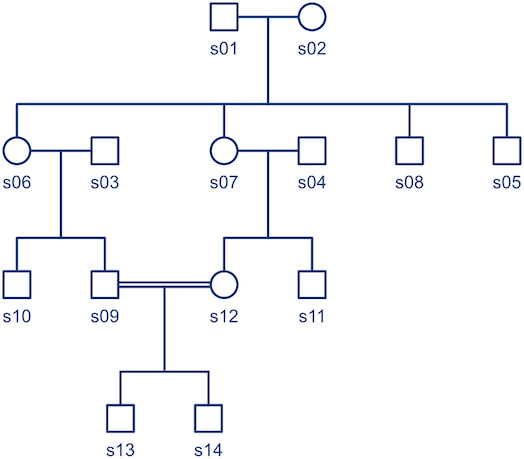
Consider the pedigree in the figure below, consisted of 14 subjects:

The corresponding kinship matrix, already multiplied by two to indicate expected covariances between subjects (i.e., $2\cdot\mathbf{\Phi}$ ), is:

Note that the diagonal elements can have values above unity, given the consanguineous mating in the family (between s09 and s12, indicated by the double line in the pedigree diagram).

In the next post, details on how the kinship matrix can be used investigate heritabilities, genetic correlations, and to perform association studies will be presented.

Genetic resemblance between relatives

Posted on 13.June.2015 by A. M. Winkler

How similar?

The degree of relationship between two related individuals can be estimated by the probability that a gene in one subject is identical by descent to the corresponding gene (i.e., in the same locus) in the other. Two genes are said to be identical by descent (ibd) if both are copies of the same ancestral gene. Genes that are not ibd may still be identical through separate mutations, and be therefore identical by state (ibs), though these will not be considered in what follows.

The coefficients below were introduced by Jacquard in 1970, in a book originally published in French, and translated to English in 1974. A similar content appeared in an article by the same author in the journal Biometrics in 1972 (see the references at the end).

Coefficients of identity

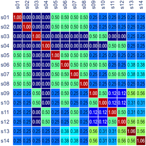
Consider a particular autosomal gene $G$ . Each individual has two copies, one from paternal, another from maternal origin; these can be indicated as $G_i^P$ and $G_i^M$ for individual $i$ . There are 15 exactly distinct ways (states) in which the $G$ can be identical or not identical between two individuals, as shown in the figure below.

To each of these states $S_{1, \ldots , 15}$ , a respective probability $\delta_{1, \ldots , 15}$ can be assigned; these are called coefficients of identity by descent. These probabilities can be calculated at every generation following very elementary rules. For most problems, however, the distinction between paternal and maternal origin of a gene is irrelevant, and some of the above states are equivalent to others. If these are condensed, we can retain 9 distinct ways, shown in the figure below:

As before, to each of these states $\Sigma_{1, \ldots , 9}$ , a respective probability $\Delta_{1, \ldots , 9}$ can be assigned; these are called condensed coefficients of identity by descent, and relate to the former as:

$\Delta_1 = \delta_1$
$\Delta_2 = \delta_6$
$\Delta_3 = \delta_2 + \delta_3$
$\Delta_4 = \delta_7$
$\Delta_5 = \delta_4 + \delta_5$
$\Delta_6 = \delta_8$
$\Delta_7 = \delta_9 + \delta_{12}$
$\Delta_8 = \delta_{10} + \delta_{11} + \delta_{13} + \delta_{14}$
$\Delta_9 = \delta_{15}$

A similar method was proposed by Cotterman (1940), in his highly influential but only much later published doctoral thesis. The $\Delta_9$ , $\Delta_8$ and $\Delta_7$ correspond to his coefficients $k_0$ , $k_1$ and $k_2$ .

Coefficient of kinship

The above refer to probabilities of finding particular genes as identical among subjects. However, a different coefficient can be defined for random genes: the probability that a random gene from subject $i$ is identical with a gene at the same locus from subject $j$ is the coefficient of kinship, and can be represented as $\phi_{ij}$ :

$\phi_{ij} = \Delta_1 + \frac{1}{2}(\Delta_3 + \Delta_5 + \Delta_7) + \frac{1}{4}\Delta_8$

If $i$ and $j$ are in fact the same individual, then $\phi_{ii}$ is the kinship of a subject with himself. Two genes taken from the same individual can either be the same gene (probability $\frac{1}{2}$ of being the same) or be the genes inherited from father and mother, in which case the probability is given by the coefficient of kinship between the parents. In other words, $\phi_{ii} = \frac{1}{2} + \frac{1}{2}\phi_{\text{FM}}$ . If both parents are unrelated, $\phi_{\text{FM}}=0$ , such that the kinship of a subject with himself is $\phi_{ii} = \frac{1}{2}$ .

The value of $\phi_{ij}$ can be determined from the number of generations up to a common ancestor $k$ . A random gene from individual $i$ can be identical to a random gene from individual $j$ in the same locus if both comes from the common ancestor $k$ , an event that can happen if either (1) both are copies of the gene in $k$ , or (2) if they are copies of different genes in $k$ , but $k$ is inbred; this has probability $\frac{1}{2}f_k$ (see below about the coefficient of inbreeding, $f$ ). Thus, if there are $m$ generations between $i$ and $k$ , and $n$ generations between $j$ and $k$ , the coefficient of kinship can be computed as $\phi_{ij} = \left(\frac{1}{2}\right)^{m+n+1}(1+f_k)$ . If $i$ and $j$ can have more than one common ancestor, then there are more than one line of descent possible, and the kinship is determined by integrating over all such possible $K$ common ancestors:

$\phi_{ij} = \sum_{k=1}^K \left(\frac{1}{2}\right)^{m_k+n_k+1}(1+f_k)$

For a set of subjects, the pairwise coefficients of kinship $\phi_{ij}$ can be arranged in a square matrix $\boldsymbol{\Phi}$ , and used to model the covariance between subjects as $2\cdot\boldsymbol{\Phi}$ (see here).

Coefficient of inbreeding

The coefficient of inbreeding $f$ of a given subject $i$ is the coefficient of kinship between their parents. While the above coefficients provide information about pairs of individuals, the coefficient of inbreeding gives information about a particular subject. Yet, $f_i$ can be computed from the coefficients of identity:

$f_{i} = \Delta_1 + \Delta_2 + \Delta_3 + \Delta_4$
$f_{j} = \Delta_1 + \Delta_2 + \Delta_5 + \Delta_6$

Note that all these coefficients are based on probabilities, but it is now possible to identify the actual presence of a particular gene using marker data. Also note that while the illustrations above suggest application to livestock, the same applies to studies of human populations.

Some particular cases

The computation of the above coefficients can be done using algorithms, and are done automatically by software that allow analyses of pedigree data, such as solar. Some common particular cases are shown below:

Relationship	$\Delta_1$	$\Delta_2$	$\Delta_3$	$\Delta_4$	$\Delta_5$	$\Delta_6$	$\Delta_7$	$\Delta_8$	$\Delta_9$	$\phi_{ij}$
Self	$0$	$0$	$0$	$0$	$0$	$0$	$1$	$0$	$0$	$\frac{1}{2}$
Parent-offspring	$0$	$0$	$0$	$0$	$0$	$0$	$0$	$1$	$0$	$\frac{1}{4}$
Half sibs	$0$	$0$	$0$	$0$	$0$	$0$	$0$	$\frac{1}{2}$	$\frac{1}{2}$	$\frac{1}{8}$
Full sibs/dizygotic twins	$0$	$0$	$0$	$0$	$0$	$0$	$\frac{1}{4}$	$\frac{1}{2}$	$\frac{1}{4}$	$\frac{1}{4}$
Monozygotic twins	$0$	$0$	$0$	$0$	$0$	$0$	$1$	$0$	$0$	$\frac{1}{2}$
First cousins	$0$	$0$	$0$	$0$	$0$	$0$	$0$	$\frac{1}{4}$	$\frac{3}{4}$	$\frac{1}{16}$
Double first cousins	$0$	$0$	$0$	$0$	$0$	$0$	$\frac{1}{16}$	$\frac{6}{16}$	$\frac{9}{16}$	$\frac{1}{8}$
Second cousins	$0$	$0$	$0$	$0$	$0$	$0$	$0$	$\frac{1}{16}$	$\frac{15}{16}$	$\frac{1}{64}$
Uncle-nephew	$0$	$0$	$0$	$0$	$0$	$0$	$0$	$\frac{1}{2}$	$\frac{1}{2}$	$\frac{1}{8}$
Offspring of sib-matings	$\frac{1}{16}$	$\frac{1}{32}$	$\frac{1}{8}$	$\frac{1}{32}$	$\frac{1}{8}$	$\frac{1}{32}$	$\frac{7}{32}$	$\frac{5}{16}$	$\frac{1}{16}$	$\frac{3}{8}$

References

Cotterman C. A calculus for statistico-genetics. 1940. PhD Thesis. Ohio State University.
Jacquard, A. Structures génétiques des populations. Masson, Paris, France, 1970, later translated and republished as Jacquard, A. The genetic structure of populations. Springer, Heidelberg, 1974.
Jacquard A. Genetic information given by a relative. Biometrics. 1972;28(4):1101-1114.

The photograph at the top (sheep) is in public domain.

All GLM formulas

Posted on 04.March.2015 by A. M. Winkler

It’s so often that we find ourselves in the need to quickly compute a statistic for a certain dataset, but finding the formulas is not always direct. Using a statistical software is helpful, but it often also happens that the reported results are not exactly what one may believe it represents. Moreover, even if using these packages, it is always good to have in mind the meaning of statistics and how they are computed. Here the formulas for the most commonly used statistics with the general linear model (glm) are presented, all in matrix form, that can be easily implemented in Octave or Matlab.

I — Model

We consider two models, one univariate, another multivariate. The univariate is a particular case of the multivariate, but for univariate problems, it is simpler to use the smaller, particular case.

Univariate model

The univariate glm can be written as:

$\mathbf{y} = \mathbf{M}\boldsymbol{\psi} + \boldsymbol{\epsilon}$

where $\mathbf{y}$ is the $N \times 1$ vector of observations, $\mathbf{M}$ is the $N \times s$ matrix of explanatory variables, $\boldsymbol{\psi}$ is the $s \times 1$ vector of regression coefficients, and $\boldsymbol{\epsilon}$ is the $N \times 1$ vector of residuals.

The null hypothesis can be stated as $\mathcal{H}_0 : \mathbf{C}'\boldsymbol{\psi} = 0$ , where $\mathbf{C}$ is a $s \times s'$ matrix that defines a contrast of regression coefficients, satisfying $\mathsf{rank}(\mathbf{C}) = s'$ and $1 \geqslant s' \geqslant s$ .

Multivariate model

The multivariate glm can be written as:

$\mathbf{Y} = \mathbf{M}\boldsymbol{\Psi} + \boldsymbol{\epsilon}$

where $\mathbf{Y}$ is the $N \times q$ vector of observations, $\mathbf{M}$ is the $N \times s$ matrix of explanatory variables, $\boldsymbol{\Psi}$ is the $s \times q$ vector of regression coefficients, and $\boldsymbol{\epsilon}$ is the $N \times q$ vector of residuals.

The null hypothesis can be stated as $\mathcal{H}_0 : \mathbf{C}'\boldsymbol{\Psi}\mathbf{D} = 0$ , where $\mathbf{C}$ is defined as above, and $\mathbf{D}$ is a $q \times q'$ matrix that defines a contrast of observed variables, satisfying $\mathsf{rank}(\mathbf{D}) = q'$ and $1 \geqslant q' \geqslant q$ .

II — Estimation of parameters

In the model, the unknowns of interest are the values arranged in $\boldsymbol{\Psi}$ . These can be estimated as:

$\boldsymbol{\hat{\Psi}} = (\mathbf{M}'\mathbf{M})^{+}(\mathbf{M}'\mathbf{Y})$

where the $^{+}$ represents a pseudo-inverse. The residuals can be computed as:

$\boldsymbol{\hat{\epsilon}} = \mathbf{Y} - \mathbf{M}\boldsymbol{\hat{\Psi}}$

The above also applies to the univariate case ( $\mathbf{y}$ is a particular case of $\mathbf{Y}$ , and $\boldsymbol{\psi}$ of $\boldsymbol{\Psi}$ ).

III – Univariate statistics

Coefficient of determination, R²

The following is the fraction of the variance explained by the part of the model determined by the contrast. It applies to mean-centered data and design, i.e., $\tilde{\mathbf{y}}=\mathbf{y}-\bar{y}$ and $\tilde{\mathbf{M}}=\mathbf{M}-\bar{\mathbf{m}}$ .

$R^2 = \dfrac{\boldsymbol{\hat{\psi}}'\mathbf{C} \left(\mathbf{C}'(\tilde{\mathbf{M}}'\tilde{\mathbf{M}})^{-1}\mathbf{C} \right)^{-1} \mathbf{C}'\boldsymbol{\hat{\psi}}}{\tilde{\mathbf{y}}'\tilde{\mathbf{y}}}$

Note that the portion of the variance explained by nuisance variables (if any) remains in the denominator. To have these taken into account, consider the squared partial correlation coefficient, or Pillai’s trace with univariate data, both described further down.

Pearson’s correlation coefficient

When $\mathsf{rank}\left(\mathbf{C}\right) = 1$ , the multiple correlation coefficient can be computed from the $R^2$ statistic as:

$R = \mathsf{sign}\left(\mathbf{C}'\boldsymbol{\hat{\psi}}\right)\sqrt{R^2}$

This value should not be confused, even in the presence of nuisance, with the partial correlation coefficient (see below).

Student’s t statistic

If $\mathsf{rank}\left(\mathbf{C}\right) = 1$ , the Student’s $t$ statistic can be computed as:

$t = \boldsymbol{\hat{\psi}}'\mathbf{C} \left(\mathbf{C}'(\mathbf{M}'\mathbf{M})^{-1}\mathbf{C} \right)^{-\frac{1}{2}} \left/ \sqrt{\dfrac{\boldsymbol{\hat{\epsilon}}'\boldsymbol{\hat{\epsilon}}}{N-\mathsf{rank}\left(\mathbf{M}\right)}} \right.$

F statistic

The $F$ statistic can be computed as:

$F = \left.\dfrac{\boldsymbol{\hat{\psi}}'\mathbf{C} \left( \mathbf{C}'(\mathbf{M}'\mathbf{M})^{-1}\mathbf{C} \right)^{-1} \mathbf{C}'\boldsymbol{\hat{\psi}}}{\mathsf{rank}\left(\mathbf{C} \right)} \right/ \dfrac{\boldsymbol{\hat{\epsilon}}'\boldsymbol{\hat{\epsilon}}}{N-\mathsf{rank}\left(\mathbf{M}\right)}$

Aspin—Welch v

If homoscedastic variances cannot be assumed, and $\mathsf{rank}\left(\mathbf{C}\right) = 1$ , this is equivalent to the Behrens—Fisher problem, and the Aspin—Welch’s $t$ statistic can be computed as:

$v = \boldsymbol{\hat{\psi}}'\mathbf{C} \left(\mathbf{C}'(\mathbf{M}'\mathbf{W}\mathbf{M})^{-1}\mathbf{C} \right)^{-\frac{1}{2}}$

where $\mathbf{W}$ is a diagonal matrix that has elements:

$W_{nn}=\dfrac{\sum_{n' \in g_{n}}R_{n'n'}}{\boldsymbol{\hat{\epsilon}}_{g_{n}}'\boldsymbol{\hat{\epsilon}}_{g_{n}}}$

and where $R_{n'n'}$ are the $n'$ diagonal elements of the residual forming matrix $\mathbf{R} = \mathbf{I}-\mathbf{M}\mathbf{M}^{+}$ , and $g_{n}$ is the variance group to which the $n$ -th observation belongs.

Generalised G statistic

If variances cannot be assumed to be the same across all observations, a generalisation of the $F$ statistic can be computed as:

$G = \dfrac{\boldsymbol{\hat{\psi}}'\mathbf{C} \left(\mathbf{C}'(\mathbf{M}'\mathbf{W}\mathbf{M})^{-1}\mathbf{C} \right)^{-1} \mathbf{C}'\boldsymbol{\hat{\psi}}}{\Lambda \cdot \mathsf{rank}\left(\mathbf{C}\right)}$

where $\mathbf{W}$ is defined as above, and the remaining denominator term, $\Lambda$ , is given by:

$\Lambda = 1+\frac{2(s-1)}{s(s+2)}\sum_{g} \frac{1}{\sum_{n \in g}R_{nn}} \left(1-\frac{\sum_{n \in g}W_{nn}}{\mathsf{trace}\left(\mathbf{W}\right)}\right)^2$

There is another post on the G-statistic (here).

Partial correlation coefficient

When $\mathsf{rank}\left(\mathbf{C}\right) = 1$ , the partial correlation can be computed from the Student’s $t$ statistic as:

$r = \mathsf{sign}\left(t\right)\sqrt{\dfrac{t^2}{N-\mathsf{rank}\left(\mathbf{M}\right)+t^2}}$

The square of the partial correlation corresponds to Pillai’s trace applied to an univariate model, and it can also be computed from the $F$ -statistic as:

$r^2 = \dfrac{F}{\frac{N-\mathsf{rank}\left(\mathbf{M}\right)}{\mathsf{rank}\left(\mathbf{C}\right)}+F}$

Likewise, if $r$ is known, the formula can be solved for $t$ :

$t = \dfrac{r\sqrt{N-\mathsf{rank}\left(\mathbf{M}\right)}}{\sqrt{1-r^2}}$

or for $F$ :

$F = \dfrac{r^2}{1-r^2}\times\dfrac{N-\mathsf{rank}\left(\mathbf{M}\right)}{\mathsf{rank}\left(\mathbf{C}\right)}$

The partial correlation can also be computed at once for all variables vs. all other variables as follows. Let $\mathbf{A} = \left[\mathbf{y}\; \mathbf{M}\right]$ , and $\mathsf{r}\left(\mathbf{A}\right)$ be the inverse of the correlation matrix of the columns of $\mathbf{A}$ , and $\mathsf{d}\left(\cdot\right)$ the diagonal operator, that returns a column vector with the diagonal entries of a square matrix. Then the matrix with the partial correlations is:

$\mathbf{r} = -\mathsf{r}\left(\mathbf{A}\right) \odot \left(\mathsf{d}\left(\mathsf{r}\left(\mathbf{A}\right)\right)\mathsf{d}\left(\mathsf{r}\left(\mathbf{A}\right)\right)'\right)^{-\frac{1}{2}}$

where $\odot$ is the Hadamard product, and the power “ $-\frac{1}{2}$ ” is taken elementwise (i.e., not matrix power).

IV – Multivariate statistics

For the multivariate statistics, define generically $\mathbf{E} = (\boldsymbol{\hat{\epsilon}}\mathbf{D})'(\boldsymbol{\hat{\epsilon}}\mathbf{D})$ as the sums of the products of the residuals, and $\mathbf{H}=(\mathbf{C}'\boldsymbol{\hat{\Psi}}\mathbf{D})' \left(\mathbf{C}'(\mathbf{M}'\mathbf{M})^{-1}\mathbf{C} \right)^{-1} (\mathbf{C}'\boldsymbol{\hat{\Psi}}\mathbf{D})$ as the sums of products of the hypothesis. In fact, the original model can be modified as $\tilde{\mathbf{Y}} = \mathbf{M}\tilde{\boldsymbol{\Psi}} + \tilde{\boldsymbol{\epsilon}}$ , where $\tilde{\mathbf{Y}}=\mathbf{Y}\mathbf{D}$ , $\tilde{\boldsymbol{\Psi}} = \boldsymbol{\Psi}\mathbf{D}$ and $\tilde{\boldsymbol{\epsilon}}=\boldsymbol{\epsilon}\mathbf{D}$ .

If $\mathsf{rank}\left(\mathbf{D}\right)=1$ , this is an univariate model, otherwise it remains multivariate, although $\mathbf{D}$ can be omitted from the formulas. From now on this simplification is adopted, so that $\mathbf{E} = \boldsymbol{\hat{\epsilon}}'\boldsymbol{\hat{\epsilon}}$ and $\mathbf{H}=\boldsymbol{\hat{\Psi}}'\mathbf{C} \left(\mathbf{C}'(\mathbf{M}'\mathbf{M})^{-1}\mathbf{C} \right)^{-1} \mathbf{C}'\boldsymbol{\hat{\Psi}}$ .

Hotelling T²

If $\mathsf{rank}\left(\mathbf{C}\right) = 1$ , the Hotelling’s $T^2$ statistic can be computed as:

$T^2 = \mathbf{C}'\boldsymbol{\hat{\Psi}}\boldsymbol{\Sigma}^{-\frac{1}{2}}\left(\mathbf{C}'(\mathbf{M}'\mathbf{M})^{-1}\mathbf{C} \right)^{-1}\boldsymbol{\Sigma}^{-\frac{1}{2}} \boldsymbol{\hat{\Psi}}'\mathbf{C}$

where $\boldsymbol{\Sigma} = \mathbf{E}/\left(N-\mathsf{rank}\left(\mathbf{M}\right)\right)$

Multivariate alternatives to the F statistic

Classical manova/mancova statistics can be based in the ratio between the sums of products of the hypothesis and the sums of products of the residuals, or the ratio between the sums of products of the hypothesis and the total sums of products. In other words, define:

$\begin{array}{ccl} \mathbf{A} &=& \mathbf{H}\mathbf{E}^{-1} = \mathbf{E}^{-\frac{1}{2}} \boldsymbol{\hat{\psi}}'\mathbf{C} \left(\mathbf{C}'(\mathbf{M}'\mathbf{M})^{-1}\mathbf{C} \right)^{-1} \mathbf{C}'\boldsymbol{\hat{\psi}}\mathbf{E}^{-\frac{1}{2}}\\ \mathbf{B} &=& \mathbf{H}\left(\mathbf{E}+\mathbf{H}\right)^{-1} \end{array}$

Let $\lambda_i$ be the eigenvalues of $\mathbf{A}$ , and $\theta_i$ the eigenvalues of $\mathbf{B}$ . Then:

Wilks’ $\Lambda = \prod_{i} \dfrac{1}{1+\lambda_i} = \dfrac{|\mathbf{E}|}{|\mathbf{E}+\mathbf{H}|}$ .
Lawley–Hotelling’s trace: $\sum_i \lambda_i = \mathsf{trace}\left(\mathbf{A}\right)$ .
Pillai’s trace: $\sum_i \dfrac{\lambda_i}{1+\lambda_i} = \sum_i \theta_i = \mathsf{trace}\left(\mathbf{B}\right)$ .
Roy’s largest root (ii): $\lambda_1 = \mathsf{max}_i\left(\lambda_i\right) = \dfrac{\theta_1}{1-\theta_1}$ (analogous to $F$ ).
Roy’s largest root (iii): $\theta_1 = \mathsf{max}_i\left(\theta_i\right) = \dfrac{\lambda_1}{1+\lambda_1}$ (analogous to $R^2$ ).

When $\mathsf{rank}\left(\mathbf{C}\right) = 1$ , or when $\mathbf{Y}$ is univariate, or both, Lawley–Hotelling’s trace is equal to Roy’s (ii) largest root, Pillai’s trace is equal to Roy’s (iii) largest root, and Wilks’ $\Lambda$ added to Pillai’s trace equals to unity. The value $\rho_i=\sqrt{\theta_i}$ is the $i$ -th canonical correlation.

References

Wilks S. Certain Generalizations in the Analysis of Variance. Biometrika. 1932;24(3):471-494.
Lawley D. A Generalization of Fisher’s z Test. Biometrika. 1938;30(1):180-187.
Hotelling H. A generalized T test and measure of multivariate dispersion. In: Neyman J, ed. Proceedings of the Second Berkeley Symposium on Mathematical Statistics and Probability. Berkeley: University of California Press; 1951:23-41.
Roy SN. On a Heuristic Method of Test Construction and its use in Multivariate Analysis. Ann Math Stat. 1953;24(2):220-238.
Pillai KCS. Some New Test Criteria in Multivariate Analysis. Ann Math Stat. 1955;26(1):117-121.
Winkler AM, Ridgway GR, Webster MA, Smith SM, Nichols TE. Permutation Inference for the general linear model. Neuroimage. 2014 May 15;92:381-97.

The G-statistic

Posted on 17.February.2014 by A. M. Winkler

Preliminaries

Consider the common analysis of a neuroimaging experiment. At each voxel, vertex, face or edge (or any other imaging unit), we have a linear model expressed as:

$\mathbf{Y} = \mathbf{M} \boldsymbol{\psi} + \boldsymbol{\epsilon}$

where $\mathbf{Y}$ contains the experimental data, $\mathbf{M}$ contains the regressors, $\boldsymbol{\psi}$ the regression coefficients, which are to be estimated, and $\boldsymbol{\epsilon}$ the residuals. For a linear null hypothesis $\mathcal{H}_0 : \mathbf{C}'\boldsymbol{\psi}=\mathbf{0}$ , where $\mathbf{C}$ is a contrast. If $\mathsf{rank}\left(\mathbf{C}\right) = 1$ , the Student’s t statistic can be calculated as:

where the hat on $\boldsymbol{\hat{\psi}}$ and $\boldsymbol{\hat{\epsilon}}$ indicate that these are quantities estimated from the sample. If $\mathsf{rank}\left(\mathbf{C}\right) \geqslant 1$ , the F statistic can be obtained as:

$F = \left.\dfrac{\boldsymbol{\hat{\psi}}'\mathbf{C} \left(\mathbf{C}'(\mathbf{M}'\mathbf{M})^{-1}\mathbf{C} \right)^{-1} \mathbf{C}'\boldsymbol{\hat{\psi}}}{\mathsf{rank}\left(\mathbf{C}\right)} \right/ \dfrac{\boldsymbol{\hat{\epsilon}}'\boldsymbol{\hat{\epsilon}}}{N-\mathsf{rank}\left(\mathbf{M}\right)}$

When $\mathsf{rank}\left(\mathbf{C}\right) = 1$ , $F = t^2$ . For either of these statistics, we can assess their significance by repeating the same fit after permuting $\mathbf{Y}$ or $\mathbf{M}$ (i.e., a permutation test), or by referring to the formula for the distribution of the corresponding statistic, which is available in most statistical software packages (i.e., a parametric test).

Permutation tests don’t depend on the same assumptions on which parametric tests are based. As some of these assumptions can be quite stringent in practice, permutation methods arguably should be preferred as a general framework for the statistical analysis of imaging data. At each permutation, a new statistic is computed and used to build its empirical distribution from which the p-values are obtained. In practice it’s not necessary to build the full distribution, and it suffices to increment a counter at each permutation. At the end, the counter is divided by the number of permutations to produce a p-value.

An example of a permutation distribution

Using permutation tests, correction for multiple testing using the family-wise error rate (fwer) is trivial: rather than build the permutation distribution at each voxel, a single distribution of the global maximum of the statistic across the image is constructed. Each permutation yields one maximum, that is used to build the distribution. Any dependence between the tests is implicitly captured, with not need to model it explicitly, nor to introduce even more assumptions, a problem that hinders methods such as the random field theory.

Exchangeability blocks

Permutation is allowed if it doesn’t affect the joint distribution of the error terms, i.e., if the errors are exchangeable. Some types of experiments may involve repeated measurements or other kinds of dependency, such that exchangeability cannot be guaranteed between all observations. However, various cases of structured dependency can still be accommodated if sets (blocks) of observations are shuffled as a whole, or if shuffling happens only within set (block). It is not necessary to know or to model the exact dependence structure between observations, which is captured implicitly as long as the blocks are defined correctly.

Permutation within block.

Permutation of blocks as a whole.

The two figures above are of designs constructed using the fsl software package. In fsl, within-block permutation is available in randomise with the option -e, used to supply a file with the definition of blocks. For whole-block permutation, in addition to the option -e, the option --permuteBlocks needs to be supplied.

The G-statistic

The presence of exchangeability blocks solves a problem, but creates another. Having blocks implies that observations may not be pooled together to produce a non-linear parameter estimate such as the variance. In other words: the mere presence of exchangeability blocks, either for shuffling within or as a whole, implies that the variances may not be the same across all observations, and a single estimate of this variance is likely to be inaccurate whenever the variances truly differ, or if the groups don’t have the same size. This also means that the F or t statistics may not behave as expected.

The solution is to use the block definitions and the permutation strategy is to define groups of observations that are known or assumed to have identical variances, and pool only the observations within group for variance estimation, i.e., to define variance groups (vgs).

The F-statistic, however, doesn’t allow such multiple groups of variances, and we need to resort to another statistic. In Winkler et al. (2014) we propose:

$G = \dfrac{\boldsymbol{\hat{\psi}}'\mathbf{C} \left(\mathbf{C}'(\mathbf{M}'\mathbf{W}\mathbf{M})^{-1}\mathbf{C} \right)^{-1} \mathbf{C}'\boldsymbol{\hat{\psi}}}{\Lambda \cdot s}$

where $\mathbf{W}$ is a diagonal matrix that has elements:

$W_{nn}=\dfrac{\sum_{n' \in g_{n}}R_{n'n'}}{\boldsymbol{\hat{\epsilon}}_{g_{n}}'\boldsymbol{\hat{\epsilon}}_{g_{n}}}$

and where $R_{n'n'}$ are the $n'$ diagonal elements of the residual forming matrix, and $g_{n}$ is the variance group to which the $n$ -th observation belongs. The remaining denominator term, $\Lambda$ , is given by (Welch, 1951):

$\Lambda = 1+\frac{2(s-1)}{s(s+2)}\sum_{g} \frac{1}{\sum_{n \in g}R_{nn}} \left(1-\frac{\sum_{n \in g}W_{nn}}{\mathsf{trace}\left(\mathbf{W}\right)}\right)^2$

where $s=\mathsf{rank}\left(\mathbf{C}\right)$ . The matrix $\mathbf{W}$ can be seen as a weighting matrix, the square root of which normalises the model such that the errors have then unit variance and can be ignored. It can also be seen as being itself a variance estimator. In fact, it is the very same variance estimator proposed by Horn et al (1975).

The W matrix used with the G statistic. It is constructed from the estimated variances of the error terms.

The matrix $\mathbf{W}$ has a crucial role in making the statistic pivotal in the presence of heteroscedasticity. Pivotality means that the statistic has a sampling distribution that is not dependent on any unknown parameter. For imaging experiments, it’s important that the statistic has this property, otherwise correction for multiple testing that controls fwer will be inaccurate, or possibly invalid altogether.

When $\mathsf{rank}\left(\mathbf{C}\right)=1$ , the t-equivalent to the G-statistic is $v = \boldsymbol{\hat{\psi}}'\mathbf{C} \left(\mathbf{C}'(\mathbf{M}'\mathbf{W}\mathbf{M})^{-1}\mathbf{C} \right)^{-\frac{1}{2}}$ , which is the well known Aspin-Welch $v$ -statistic for the Behrens-Fisher problem. The relationship between $v$ and G is the same as between t and F, i.e., when the rank of the contrast equals to one, the latter is simply the square of the former. The G statistic is a generalization of all these, and more, as we show in the paper, and summarise in the table below:

	$\mathsf{rank}\left(\mathbf{C}\right) = 1$	$\mathsf{rank}\left(\mathbf{C}\right) > 1$
Homoscedastic errors, unrestricted exchangeability	Square of Student’s t	F-ratio
Homoscedastic within vg, restricted exchangeability	Square of Aspin-Welch $v$	Welch’s $v^2$

In the absence of variance groups (i.e., all observations belong to the same vg), G and $v$ are equivalent to F and t respectively.

Although not typically necessary if permutation methods are to be preferred, approximate parametric p-values for the G-statistic can be computed from an F-distribution with $\nu_1=s$ and $\nu_2=2(s-1)/3/(\Lambda-1)$ .

While the error rates are controlled adequately (a feature of permutation tests in general), the G-statistic offers excellent power when compared to the F-statistic, even when the assumptions of the latter are perfectly met. Moreover, by preserving pivotality, it is an adequate statistic to control of the error rate in the in the presence of multiple tests.

In this post, the focus is in using G for imaging data, but of course, it can be used for any dataset in which a linear model where variances cannot be assumed to be the same is used, i.e., when heteroscedasticity is or could be present.

Note that the G-statistic has nothing to do with the G-test. It is named as this for being a generalisation over various tests, including the commonly used t and F tests, as shown above.

Main reference

The core reference and results for the G-statistic have just been published in Neuroimage:

Winkler AM, Ridgway GR, Webster MA, Smith SM, Nichols TE. Permutation inference for the general linear model. Neuroimage. 2014;92:381-397

Other references

The two other references cited, which are useful to understand the variance estimator and the parametric approximation are:

Horn S, Horn R, Duncan D. Estimating heteroscedastic variances in linear models. J Am Stat Assoc. 1975;70(350):380–385.
Welch B. On the comparison of several mean values: an alternative approach. Biometrika. 1951;38(3):330–336.

Biased, as it should be

Posted on 12.April.2013 by A. M. Winkler

When we run a permutation test, what we do is to first compute the statistic for the unpermuted model, then shuffle the data randomly, compute a new statistic and, if it is larger than the statistic for the unpermuted model, increment a counter. We then repeat the random shuffling, and keep incrementing the counter until we think we are done with them. We then divide the counter by the number of permutations and the result is the p-value what we wanted to find.

This procedure can be stated as:

$\hat{p} = \frac{1}{N}\sum^{N}_{n=1}\mathcal{I}(T^{*}_{n} \geqslant T_0)$

where $\hat{p}$ is the estimated p-value, $N$ is the number of permutations, $T_0$ is the statistic for the unpermuted model, $T^{*}_n$ is the statistic for the $n$ -th random shuffling, and $\mathcal{I}$ is an indicator function that evaluates as 1 if the condition between parenthesis is true, or 0 otherwise. This formulation produces unbiased results: since $E(\mathcal{I}(T^{*}_{n} \geqslant T_0)) = p$ , the true p-value, then $E(\frac{1}{N}\sum^{N}_{n=1}\mathcal{I}(T^{*}_{n} \geqslant T_0)) = p$ .

The problem

This strategy, however, has a problem. If the true p-value, $p$ , is small, or if the number of permutations is not sufficiently large, even after all the $N$ permutations are done, no $T^{*}_{n}$ may reach or surpass the value of $T_0$ , resulting in a p-value equal to 0. While this is still a valid, unbiased result, p-values equal to zero are problematic, as they can be interpreted as indicating the rejection of the null-hypothesis with absolute confidence. And this even after very few permutations (perhaps just 1!) have been performed, which is indeed rather counter-intuitive. We cannot be completely sure of the rejection of the null simply for having done just a few permutations.

Biasing to solve the problem

The solution is to make two modifications to the formulation above: start counting the $n$ -th permutation at 0, for the unpermuted model, and divide the counter at the end not by $N$ , but by $N+1$ :

$\hat{p} = \frac{1}{N+1}\sum^{N}_{n=0}\mathcal{I}(T^{*}_{n} \geqslant T_0)$

This formulation, which pools the unpermuted model together with the permuted realisations, is biased: for $n=0$ , $\mathcal{I}(T^{*}_{n} \geqslant T_0) = 1$ , and so, $E(\frac{1}{N+1}\sum^{N}_{n=0}\mathcal{I}(T^{*}_{n} \geqslant T_0)) = \frac{1+Np}{N+1} \neq p$ .

Quantifying the bias

The bias is smaller for a large number of permutations, and converges to zero as $N$ increases towards infinity. What is important, however, is that the bias punishes the results towards conservativeness whenever the true and unknown $p$ is smaller than $\frac{1}{N+1}$ , in a way that no p-value smaller than $\frac{1}{N+1}$ can ever be attained. It forces the researcher to run more permutations to find such small p-values to reject the null hypothesis, which otherwise could be rejected with a p-value equal to zero that would appear easily even after just a handful of permutations.

The bias is larger for smaller number of permutations and for smaller true p-values.

Controversy

The solution has been proposed by some authors, such as Edgington (1995), and strongly advocated by, e.g., Phipson and Smyth (2010). While the biased solution is definitely the most adequate for practical scientific problems, it can be considered as of little actual statistical meaning. Pesarin and Salmaso (2010) explain that the distribution of $T_0$ is not the same as the distribution of $T^{*}_{n}$ , unless the null is true. Under the alternative hypothesis, therefore, $T_0$ should not be pooled into the empirical distribution from which the p-value is obtained. Moreover, under the null, all possible permutations have the same probability, with no intrinsic reason to treat some (as the unpermuted) differently than others. If one wants unbiased results, the alternative formulation should obviously not be used.

References

Edgington ES. Randomization Tests. 3rd ed. Dekker, 1995.
Pesarin F and Salmaso L. Permutation Tests for Complex Data. Wiley, 2010.
Phipson B and Smith GK. Permutation P-values should never be zero: calculating exact P-values when permutations are randomly drawn. Stat Appl Genet Mol Biol. 2010;9:Article39.

Competition ranking and empirical distributions

Posted on 28.November.2012 by A. M. Winkler

Estimating the empirical cumulative distribution function (empirical cdf) from a set of observed values requires computing, for each value, how many of the other values are smaller or equal to it. In other words, let $X = \{x_1, x_2, \ldots , x_N\}$ be the observed values, then:

$F(x) = P(X \leqslant x) = \frac{1}{N} \sum_{n=1}^{N}I(x_n \leqslant x)$

where $F(x)$ is the empirical cdf, $P(X \leqslant x)$ is the probability of observing a value in $X$ that is smaller than or equal to $x$ , $I(\cdot)$ is a function that evaluates as 1 if the condition in the parenthesis is satisfied or 0 otherwise, and $N$ is the number of observations. This definition is straightforward and can be found in many statistical textbooks (see, e.g., Papoulis, 1991).

For continuous distributions, a p-value for a given $x \in X$ can be computed as $1-F(x)$ . For a discrete cdf, however, this trivial relationship does not hold. The reason is that, while for continuous distributions the probability $P(X = x) = 0$ , for discrete distributions (such as empirical distributions), $P(X = x) > 0$ whenever $x \in X$ . As we often want to assign a probability to one of the values that have been observed, the condition $x \in X$ always holds, and the simple relationship between the cdf and the p-value is lost. The solution, however, is still simple: a p-value can be obtained from the cdf as $1-F(x) + 1/N$ .

In the absence of repeated values (ties), the cdf can be obtained computationally by sorting the observed data in ascending order, i.e., $X_{s} = \{x_{(1)}, x_{(2)}, \ldots , x_{(N)}\}$ . Then $F(x)=(n_x)/N$ , where $(n_x)$ represents the ascending rank of $x$ . Likewise, the p-value can be obtaining by sorting the data in descending order, and using a similar formula, $P(X \geqslant x) = (\tilde{n}_x)/N$ , where $(\tilde{n}_x)$ represents the descending rank of $x$ .

Example 1: Consider the following sequence of 10 observed values, already sorted in ascending order:

$X=\{75, 76, 79, 80, 84, 85, 86, 88, 90, 94\}$

The corresponding ranks are simply 1, 2, 3, 4, 5, 6, 7, 8, 9, 10. Consequently, the cdf is:

$F(x|x\in X) = \{0.1, 0.2, 0.3, 0.4, 0.5, 0.6, 0.7, 0.8, 0.9, 1\}$

The p-values are computed by using the ranks in descending order, i.e., 10, 9, 8, 7, 6, 5, 4, 3, 2, 1, which yields:

$P(X \geqslant x | x \in X) = \{1, 0.9, 0.8, 0.7, 0.6, 0.5, 0.4, 0.3, 0.2, 0.1\}$

The problem with ties

Simple sorting, as above, is effective when there are no repeated values in the data. However, in the presence of ties, simple sorting that produces ordinal rankings yield incorrect results.

Example 2: Consider the following sequence of 10 observed values, in which ties are present:

$X = \{81, 81, 82, 83, 83, 83, 84, 85, 85, 85\}$

If the same computational strategy discussed above were used, the we would conclude that the p-value for $x=85$ would be either 0.1, 0.2 or 0.3, depending on which instance of the “85” we were to choose. The correct value, however, is 0.3 (only), since 3 out of 10 variables are equal or above 85. The solution to this problem is to replace the simple, ordinal ranking, for a modified version of the so called competition ranking.

The competition ranking

The competition ranking assigns the same rank to values that are identical. The standard competition ranking for the previous sequence is, in ascending order, 1, 1, 3, 4, 4, 4, 7, 8, 8, 8. In descending order, the ranks are 9, 9, 8, 5, 5, 5, 4, 1, 1, 1. Note that in this ranking, the ties receive the “best” possible rank. A slightly different approach consists in assigning the “worst” possible rank to the ties. This modified competition ranking applied the previous sequence gives, in ascending order, the ranks 2, 2, 3, 5, 5, 5, 7, 10, 10, 10, whereas in descending order, the ranks are 10, 10, 8, 7, 7, 7, 4, 3, 3, 3.

Competition ranking solves the problem with ties for both the empirical cdf and for the calculation of the p-values. In both cases, it is the modified version of the ranking that needs to be used, i.e., the ranking that assigns the worst rank to identical values. Still using the same sequence as example, the cdf is given by:

$F(x|x\in X) = \{0.2, 0.2, 0.3, 0.6, 0.6, 0.6, 0.7, 1, 1, 1\}$

and the p-values are given by:

$P(X \geqslant x | x \in X) = \{1, 1, 0.8, 0.7, 0.7, 0.7, 0.4, 0.3, 0.3, 0.3\}$

Note that, as in the case with no ties, the p-values cannot be computed simply as $1-F(x)$ from the cdf as it would for continuous distributions. The correct formula is $1-F(x)+(n_x)/N$ , with $(n_x)$ here representing the frequency of $x$ .

Uses

The cdf of a set of observed data is useful in many types of non-parametric inference, particularly those that use bootstrap, jack-knife, Monte Carlo, or permutation tests. Ties can be quite common when working with discrete data and discrete explanatory variables using any of these methods.

References

Papoulis A. Probability, Random Variables and Stochastic Processes. McGraw-Hill, New York, 3rd ed, 1991.