Very often we find ourselves handling large matrices and, for multiple different reasons, may want or need to reduce the dimensionality of the data by retaining the most relevant principal components. A question that arises then is how many such principal components should be retained? That is, what are the principal components that provide information that can be distinguished from variability that is indistinguishable from random noise?

One simple heuristic method is the scree plot (Cattell, 1966): one computes the singular values of the matrix, plots them in descending order, and visually looks for some kind of “elbow” (or the starting point of the “scree”) to be used as a threshold. Those singular vectors (principal components) that have corresponding singular values larger than that threshold are retained, otherwise discarded. Unfortunately, the scree test is too subjective, and worse, many realistic problems can produce matrices that have multiple such “elbows”.

Many other methods to help select the number of principal components to retain exist. Some, for example, are based on information theory, or on probabilistic formulations, or on hard thresholds related the size of the matrix or the (explained) variance from the data. In this article, the little known Wachter method (Wachter, 1976) is presented.

Let be a matrix of random values with zero mean and variance . The density of the bulk spectrum of the singular values , , , of is:

and a point mass at the origin if , where , , and (Bai, 1999). This is the Marčenko and Pastur (1967) distribution. The cumulative distribution function (cdf) can be obtained by integration, i.e., . MATLAB/Octave functions that compute the cdf and its inverse are here: mpcdf.m and mpinv.m.

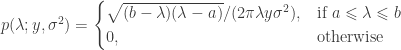
If we know the probability of finding a singular value or larger for a random matrix, we have the means to judge whether that is sufficiently large to be considered interesting enough for its corresponding singular vector (principal component) to be retained. Simply computing the p-value, however, is not enough, because the distribution makes no reference to the position of the sorted singular values. A different procedure needs be considered.

The core idea of the Wachter method is to use a QQ plot of the observed singular values versus the quantiles obtained from the inverse cdf of the Marčenko–Pastur distribution, and use eventual deviations from the identity line to help finding the threshold that separates the “good” from the “unnecessary” principal components. That is, plot the eigenvalues versus the quantiles . Deviations from the identity line are evidence for excess variance not expected from random variables alone.

The function wachter.m computes the singular values from a given observed matrix , the expected singular values should be a random matrix, as well as the p-values for each singular value in either case. The observed and expected singular values can be used to built a QQ-plot. The p-values can be used for a comparison, e.g., via the logarithm of their ratio. For example:

% For reproducibility, reset the random number generator.
% Use "rand" instead of "rng" to ensure compatibility with old versions.
rand('seed',0);

% Simulate data. See Gavish and Donoho (2014) for this example.
X = diag([1.7 2.5 zeros(1,98)]) + randn(100)*sqrt(.01); 

% Compute the expected and observed singular values,
% as well as the respective cumulative probabilities (p-values).
% See the help of wachter.m for syntax.
[Exp,Obs,Pexp,Pobs] = wachter(X,[],false,true);

% Log of the ratio between observed and expected p-values.
% Large values are evidence for "good" components.
P_ratio = -log10(Pobs./Pexp);

% Plot the spectrum.
subplot(1,2,1);
plot(Obs,'x:');
title('Singular values');
xlabel('index (k)');

% Construct the QQ-plot.
subplot(1,2,2);
qqplot(Exp,Obs);
title('QQ plot');

The result is:

In this example, two of the singular values can be considered “good”, and should be retained. The others can, according to this criterion, be dropped.

The function can take into account nuisance variables (provided in the 2nd argument), including intercept (for mean-centering), allows normalization of columns to unit variance, and can operate on p-values (upper tail from the density function) or on the cumulative probabilities. See the help text inside the function for usage information.

References

• Bai ZD. Methodologies in spectral analysis of large dimensional random matrices, a review. Statistica Sinica. 1999;9(3):611–77.
• Cattell RB. The scree test for the number of factors. Multivariate Behavioral Research. 1966;1(2):245–276.
• Gavish M, Donoho DL. The optimal hard threshold for singular values is 4/sqrt(3). arXiv:13055870. 2014.
• Johnstone IM. On the distribution of the largest eigenvalue in principal components analysis. The Annals of Statistics. 2001;29(2):295–327.
• Marčenko VA, Pastur LA. Distribution of eigenvalues for some sets of random matrices. Math USSR Sb. 1967;1(4):457–83.
• Wachter KW. Probability plotting points for principal components. In: Proceedings of the Ninth Interface Symposium on Computer Science and Statistics. Harvard University and Massachussetts Institute of Technology: Prindle, Weber & Schmidt; 1976. p. 299–308.

The image at the top is of the Drei Zinnen, in the Italian Alps during the Summer, in which a steep slope scattered with small stones (scree) is visible. Photo by Heinz Melion from Pixabay.