A higher Octave for PALM

PALM — Pemutation Analysis of Linear Models — uses either MATLAB or Octave behind the scenes. It can be executed from within either of these environments, or from the shell, in which case either of these is invoked, depending on how PALM was configured.

For users who do not want or cannot spend thousands of dollars in MATLAB licenses, Octave comes for free, and offers quite much the same benefits. However, for Octave, some functionalities in PALM require version 4.4.1 or higher. However, stable Linux distributions such as Red Hat Enterprise Linux and related (such as CentOS and Scientific Linux) still offer only 3.8.2 in the official repositories at the time of this writing, leaving the user with the task of finding an unofficial package or compiling from the source. The latter task, however, can be daunting: Octave is notoriously difficult to compile, with a myriad of dependencies.

A much simpler approach is to use Flatpak or Snappy. These are systems for distribution of Linux applications. Snappy is sponsored by Canonical (that maintains Ubuntu), whereas Flatpak appears to be the preferred tool for Fedora and openSUSE. Using either system is quite simple, and here the focus is on Flatpak.

To have a working installation of Octave, all that needs be done is:

1) Make sure Flatpak is installed:

On a RHEL/CentOS system, use (as root):

yum install flatpak

For openSUSE, use (as root):

zypper install flatpak

For Ubuntu and other Debian-based systems:

sudo apt install flatpak

2) Add the Flathub repository:

flatpak remote-add --if-not-exists flathub https://flathub.org/repo/flathub.flatpakrepo

3) Install Octave:

flatpak install flathub org.octave.Octave

4) Run it!

flatpak run org.octave.Octave

Only the installation of Flatpak needs be done as root. Once it has been installed, repositories and applications (such as Octave, among many others) can be installed at the user level. These can also be installed and made available system-wide (if run as root).

Configuring PALM

From version alpha117 onwards, the executable file ‘palm’ (not to be confused with ‘palm.m’) will include a variable named “OCTAVEBIN”, which specifies how Octave should be called. Change it from the default:

OCTAVEBIN=/usr/bin/octave

so that it invokes the version installed with Flatpak:

OCTAVEBIN="/usr/bin/flatpak run org.octave.Octave"

After making the above edits, it should be possible to run PALM directly from the system shell using the version installed via Flatpak. Alternatively, it should also be possible to invoke Octave (as in step 4 above), then use the command “addpath” to specify the location of palm.m, and then call PALM from the Octave prompt.

Octave packages

Handling of packages when Octave is installed via Flatpak is the same as usual, that is, via the command ‘pkg’ run from within Octave. More details here.

The “Group” indicator in FSL

In FSL, when we create a design using the graphical interface in FEAT, or with the command Glm, we are given the opportunity to define, at the higher-level, the “Group” to which each observation belongs. When the design is saved, the information from this setting is stored in a text file named something as “design.grp”. This file, and thus the group setting, takes different roles depending whether the analysis is used in FEAT itself, in PALM, or in randomise.

What can be confusing sometimes is that, in all three cases, the “Group” indicator does not refer to experimental or observational group of any sort. Instead, it refers to variance groups (VG) in FEAT, to exchangeability blocks (EB) in randomise, and to either VG or EB in PALM, depending on whether the file is supplied with the options -vg or -eb.

In FEAT, unless there is reason to suspect (or assume) that the variances for different observations are not equal, all subjects should belong to group “1”. If variance groups are defined, then these are taken into account when the variances are estimated. This is only possible if the design matrix is “separable”, that is, it must be such that, if the observations are sorted by group, the design can be constructed by direct sum (i.e., block-diagonal concatenation) of the design matrices for each group separately. A design is not separable if any explanatory variable (EV) present in the model crosses the group borders (see figure below). Contrasts, however, can encompass variables that are defined across multiple VGs.

The variance groups not necessarily must match the experimental observational groups that may exist in the design (for example, in a comparison of patients and controls, the variance groups may be formed based on the sex of the subjects, or another discrete variable, as opposed to the diagnostic category). Moreover, the variance groups can be defined even if all variables in the model are continuous.

In randomise, the same “Group” setting can be supplied with the option -e design.grp, thus defining exchangeability blocks. Observations within a block can only be permuted with other observations within that same block. If the option --permuteBlocks is also supplied, then the EBs must be of the same size, and the blocks as a whole are instead then permuted. Randomise does not use the concept of variance group, and all observations are always members of the same single VG.

In PALM, using -eb design.grp has the same effect that -e design.grp has in randomise. Further using the option -whole is equivalent to using --permuteBlocks in randomise. It is also possible to use together -whole and -within, meaning that the blocks as a whole are shuffled, and further, observations within block are be shuffled. In PALM the file supplied with the option -eb can have multiple columns, indicating multi-level exchangeability blocks, which are useful in designs with more complex dependence between observations. Using -vg design.grp causes PALM to use the v– or G-statistic, which are replacements for the t– and F-statistics respectively for the cases of heterogeneous variances. Although VG and EB are not the same thing, and may not always match each other, the VGs can be defined from the EBs, as exchangeability implies that some observations must have same variance, otherwise permutations are not possible. The option -vg auto defines the variance groups from the EBs, even for quite complicated cases.

In both FEAT and PALM, defining VGs will only make a difference if such variance groups are not balanced, i.e., do not have the same number of observations, since heteroscedasticity (different variances) only matter in these cases. If the groups have the same size, all subjects can be allocated to a single VG (e.g., all “1”).

Better statistics, faster

Faster permutation inference

Permutation tests are more robust and help to make scientific results more reproducible by depending on fewer assumptions. However, they are computationally intensive as recomputing a model thousands of times can be slow. The purpose of this post is to briefly list some options available for speeding up permutation.

Firstly, no speed-ups may be needed: for small sample sizes, or low resolutions, or small regions of interest, a permutation test can run in a matter of minutes. For larger data, however, accelerations may be of use. One option is acceleration through parallel processing or GPUs (for example applications of the latter, see Eklund et al., 2012, Eklund et al., 2013 and Hernández et al., 2013; references below), though this does require specialised implementation. Another option is to reduce the computational burden by exploiting the properties of the statistics and their distributions. A menu of options includes:

  • Do few permutations (shorthand name: fewperms). The results remain valid on average, although the p-values will have higher variability.
  • Keep permuting until a fixed number of permutations with statistic larger than the unpermuted is found (a.k.a., negative binomial; shorthand name: negbin).
  • Do a few permutations, then approximate the tail of the permutation distribution by fitting a generalised Pareto distribution to its tail (shorthand name: tail).
  • Approximate the permutation distribution with a gamma distribution, using simple properties of the test statistic itself, amazingly not requiring any permutations at all (shorthand name: noperm).
  • Do a few permutations, then approximate the full permutation distribution by fitting a gamma distribution (shorthand name: gamma).
  • Run permutations on only a few voxels, then fill the missing ones using low-rank matrix completion theory (shorthand name: lowrank).

These strategies allow accelerations >100x, yielding nearly identical results as in the non-accelerated case. Some, such as tail approximation, are generic enough to be used nearly all the most common scenarios, including univariate and multivariate tests, spatial statistics, and for correction for multiple testing.

In addition to accelerating permutation tests, some of these strategies, such as tail and noperm, allow continuous p-values to be found, and refine the p-values far into the tail of the distribution, thus avoiding the usual discreteness of p-values, which can be a problem in some applications if too few permutations are done.

These methods are available in the tool PALM — Permutation Analysis of Linear Models — and the complete description, evaluation, and application to the re-analysis of a voxel-based morphometry study (Douaud et al., 2007) have been just published in Winkler et al., 2016 (for the Supplementary Material, click here). The paper includes a flow chart prescribing these various approaches for each case, reproduced below.

Faster permutation inference

The hope is that these accelerations will facilitate the use of permutation tests and, if used in combination with hardware and/or software improvements, can further expedite computation leaving little reason not to use these tests.

References

Contributed to this post: Tom Nichols, Ged Ridgway.

Three HCP utilities

If you are working with data from the Human Connectome Project (HCP), perhaps these three small Octave/MATLAB utilities may be of some use:

  • hcp2blocks.m: Takes the restricted file with information about kinship and zygosity and produces a multi-level exchangeability blocks file that can be used with PALM for permutation inference. It is fully described here.
  • hcp2solar.m: Takes restricted and unrestricted files to produce a pedigree file that can be used with SOLAR for heritability and genome-wide association analyses.
  • picktraits.m: Takes either restricted or unrestricted files, a list of traits and a list of subject IDs to produce tables with selected traits for the selected subjects. These can be used to, e.g., produce design matrices for subsequent analysis.

These functions need to parse relatively large CSV files, which is somewhat inefficient in MATLAB and Octave. Still, since these commands usually have to be executed only once for a particular analysis, a 1-2 minute wait seems acceptable.

If downloaded directly from the above links, remember also to download the prerequisites: strcsvread.m and strcsvwrite.m. Alternatively, clone the full repository from GitHub. The link is this. Other tools may be added in the future.

A fourth utility

For the HCP-S1200 release (March/2017), zygosity information is provided in the fields ZygositySR (self-reported zygosity) and ZygosityGT (zygosity determined by genetic methods for select subjects). If needed, these two fields can be merged into a new field named simply Zygosity. To do so, use a fourth utility, command mergezyg.

Extreme value notes

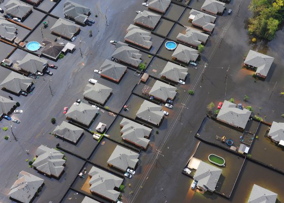
Extreme values are useful to quantify the risk of catastrophic floods, and much more.

This is a brief set of notes with an introduction to extreme value theory. For reviews, see Leadbetter et al (1983) and David and Huser (2015) [references at the end]. Also of some (historical) interest might be the classical book by Gumbel (1958). Let X_1, \dots, X_n be a sequence of independent and identically distributed variables with cumulative distribution function (cdf) F(x) and let M_n =\max(X_1,\dots,X_n) denote the maximum.

If F(x) is known, the distribution of the maximum is:

\begin{array}{lll} P(M_n \leqslant x) &=&P(X_1 \leqslant x, \dots, X_n \leqslant x) \\ &=& P(X_1 \leqslant x) \cdots P(X_n \leqslant x) = F^n(x). \end{array}

The distribution function F(x) might, however, not be known. If data are available, it can be estimated, although small errors on the estimation of F(x) can lead to large errors concerning the extreme values. Instead, an asymptotic result is given by the extremal types theorem, also known as Fisher-Tippett-Gnedenko Theorem, First Theorem of Extreme Values, or extreme value trinity theorem (called under the last name by Picklands III, 1975).

But before that, let’s make a small variable change. Working with M_n directly is problematic because as n \rightarrow \infty, F^n(x) \rightarrow 0. Redefining the problem as a function of M_n^* = \frac{M_n-b_n}{a_n} renders treatment simpler. The theorem can be stated then as: If there exist sequences of constants a_n \in \mathbb{R}_{+} and b_n \in \mathbb{R} such that, as n \rightarrow \infty:

P\left(M_{n}^{*} \leqslant x \right) \rightarrow G(x)

then G(x) belongs to one of three “domains of attraction”:

  • Type I (Gumbel law): \Lambda(x) = e^{-e^{-\frac{x-b}{a}}}, for x \in \mathbb{R} indicating that the distribution of M_n has an exponential tail.
  • Type II (Fréchet law): \Phi(x) = \begin{cases} 0 & x\leqslant b \\ e^{-\left(\frac{x-b}{a}\right)^{-\alpha}} & x\; \textgreater\; b \end{cases} indicating that the distribution of M_n has a heavy tail (including polynomial decay).
  • Type III (Weibull law): \Psi(x) = \begin{cases} e^{-\left( -\frac{x-b}{a}\right)^\alpha} & x\;\textless\; b \\ 1 & x\geqslant b \end{cases} indicating that the distribution of M_n has a light tail with finite upper bound.

Note that in the above formulation, the Weibull is reversed so that the distribution has an upper bound, as opposed to a lower one as in the Weibull distribution. Also, the parameterisation is slightly different than the one usually adopted for the Weibull distribution.

These three families have parameters a\; \textgreater\; 0, b and, for families II and III, \alpha\; \textgreater\; 0. To which of the three a particular F(x) is attracted is determined by the behaviour of the tail of of the distribution for large x. Thus, we can infer about the asymptotic properties of the maximum while having only a limited knowledge of the properties of F(x).

These three limiting cases are collectively termed extreme value distributions. Types II and III were identified by Fréchet (1927), whereas type I was found by Fisher and Tippett (1928). In his work, Fréchet used M_n^* = \frac{M_n}{a_n}, whereas Fisher and Tippett used M_n^* = \frac{M_n-b_n}{a_n}. Von Mises (1936) identified various sufficient conditions for convergence to each of these forms, and Gnedenko (1943) established a complete generalisation.

Generalised extreme value distribution

As shown above, the rescaled maxima converge in distribution to one of three families. However, all are cases of a single family that can be represented as:

G(x) = e^{-\left(1-\xi\left(\frac{x-\mu}{\sigma}\right)\right)^{\frac{1}{\xi}}}

defined on the set \left\{x:1-\xi\frac{x-\mu}{\sigma}\;\textgreater\;0\right\}, with parameters -\infty \;\textless \;\mu\;\textless\; \infty (location), \sigma\;\textgreater\;0 (scale), and -\infty\;\textless\;\xi\;\textless\;\infty (shape). This is the generalised extreme value (GEV) family of distributions. If \xi \rightarrow 0, it converges to Gumbel (type I), whereas if \xi < 0 it corresponds to Fréchet (type II), and if \xi\;\textgreater\;0 it corresponds to Weibull (type III). Inference on \xi allows choice of a particular family for a given problem.

Generalised Pareto distribution

For u\rightarrow\infty, the limiting distribution of a random variable Y=X-u, conditional on X \;\textgreater\; u, is:

H(y) = 1-\left(1-\frac{\xi y}{\tilde{\sigma}}\right)^{\frac{1}{\xi}}

defined for y \;\textgreater\; 0 and \left(1-\frac{\xi y}{\tilde{\sigma}}\right) \;\textgreater\; 0. The two parameters are the \xi (shape) and \tilde{\sigma} (scale). The shape corresponds to the same parameter \xi of the GEV, whereas the scale relates to the scale of the former as \tilde{\sigma}=\sigma-\xi(u-\mu).

The above is sometimes called the Picklands-Baikema-de Haan theorem or the Second Theorem of Extreme Values, and it defines another family of distributions, known as generalised Pareto distribution (GPD). It generalises an exponential distribution with parameter \frac{1}{\tilde{\sigma}} as \xi \rightarrow 0, an uniform distribution in the interval \left[0, \tilde{\sigma}\right] when \xi = 1, and a Pareto distribution when \xi \;\textgreater\; 0.

Parameter estimation

By restricting the attention to the most common case of -\frac{1}{2}<\xi<\frac{1}{2}, which represent distributions approximately exponential, parametters for the GPD can be estimated using at least three methods: maximum likelihood, moments, and probability-weighted moments. These are described in Hosking and Wallis (1987). For \xi outside this interval, methods have been discussed elsewhere (Oliveira, 1984). The method of moments is probably the simplest, fastest and, according to Hosking and Wallis (1987) and Knijnenburg et al (2009), has good performance for the typical cases of -\frac{1}{2}<\xi<\frac{1}{2}.

For a set of extreme observations, let \bar{x} and s^2 be respectively the sample mean and variance. The moment estimators of \tilde{\sigma} and \xi are \hat{\tilde{\sigma}} = \frac{\bar{x}}{2}\left(\frac{\bar{x}^2}{s^2}+1\right) and \hat{\xi}=\frac{1}{2}\left(\frac{\bar{x}^2}{s^2}-1\right).

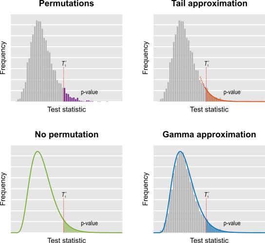
The accuracy of these estimates can be tested with, e.g., the Anderson-Darling goodness-of-fit test (Anderson and Darling, 1952; Choulakian and Stephens, 2001), based on the fact that, if the modelling is accurate, the p-values for the distribution should be uniformly distributed.

Availability

Statistics of extremes are used in PALM as a way to accelerate permutation tests. More details to follow soon.

References

The figure at the top (flood) is in public domain.

Permutation tests in the Human Connectome Project

Permutation tests are known to be superior to parametric tests: they are based on only few assumptions, essentially that the data are exchangeable, and allow the correction for the multiplicity of tests and the use of various non-standard statistics. The exchangeability assumption allows data to be permuted whenever their joint distribution remains unaltered. Usually this means that each observation needs to be independent from the others.

In many studies, however, there are repeated measurements on the same subjects, which violates exchangeability: clearly, the various measurements obtained from a given subject are not independent from each other. In the Human Connectome Project (HCP) (Van Essen et al, 2012; 2013; see references at the end), subjects are sampled along with their siblings (most of them are twins), such that independence cannot be guaranteed either.

In Winkler et al. (2014), certain structured types of non-independence in brain imaging were addressed through the definition of exchangeability blocks (EBs). Observations within EB can be shuffled freely or, alternatively, the EBs themselves can be shuffled as a whole. This allows various designs that otherwise could not be assessed through permutations.

The same idea can be generalised for blocks that are nested within other blocks, in a multi-level fashion. In the paper Multi-level Block Permutation (Winkler et al., 2015) we presented a method that allows blocks to be shuffled a whole, and inside them, sub-blocks are further allowed to be shuffled, in a recursive process. The method is flexible enough to accommodate permutations, sign-flippings (sometimes also called “wild bootstrap”), and permutations together with sign-flippings.

In particular, this permutation scheme allows the data of the HCP to be analysed via permutations: subjects are allowed to be shuffled with their siblings while keeping the joint distribution intra-sibship maintained. Then each sibship is allowed to be shuffled with others of the same type.

In the paper we show that the error type I is controlled at the nominal level, and the power is just marginally smaller than that would be obtained by permuting freely if free permutation were allowed. The more complex the block structure, the larger the reductions in power, although with large sample sizes, the difference is barely noticeable.

Importantly, simply ignoring family structure in designs as this causes the error rates not to be controlled, with excess false positives, and invalid results. We show in the paper examples of false positives that can arise, even after correction for multiple testing, when testing associations between cortical thickness, cortical area, and measures of body size as height, weight, and body-mass index, all of them highly heritable. Such false positives can be avoided with permutation tests that respect the family structure.

The figure at the top shows how the subjects of the HCP (terminal dots, shown in white colour) can be shuffled or not, while respecting the family structure. Blue dots indicate branches that can be permuted, whereas red dots indicate branches that cannot (see the main paper for details). This diagram includes 232 subjects of an early public release of HCP data. The tree on the left considers dizygotic twins as a category on their own, i.e., that cannot be shuffled with ordinary siblings, whereas the tree on the right considers dizygotic twins as ordinary siblings.

The first applied study using our strategy has just appeared. The method is implemented in the freely available package PALM — Permutation Analysis of Linear Models, and a set of practical steps to use it with actual HCP data is available here.

References