NiDB is a light, powerful, and simple to use neuroimaging database. One of its main strengths is that it was developed using a stack of stable and proven technologies: Linux, Apache, MySQL/MariaDB, PHP, and Perl. None of these technologies are new, and the fact that they have been around for so many years means that there is a lot of documentation and literature available, as well as a myriad of libraries (for PHP and Perl) that can do virtually anything. Although both PHP and Perl have received some degree of criticism (not unreasonably), and in some cases are being replaced by tools such as Node.js and Python, the volume of information about them means it is easy to find solutions when problems appear.
This article covers installation steps for either CentOS or RHEL 7, but similar steps should work with other distributions since the overall strategy is the same. By separating apart each of the steps, as opposed to doing all the configuration and installation as a single script, it becomes easier to adapt to different systems, and to identify and correct problems that may arise due to local particularities. The steps below are derived from the scripts setup-centos7.sh and setup-ubuntu16.sh, that are available in the NiDB repository, but here these will be ignored. Note that the instructions below are not “official”; for the latter, consult the NiDB documentation. The intent of this article is to facilitate the process and mitigate some frustration you may feel if trying to do it all by yourself. Also, by looking at the installation steps, you should be able to have a broad overview of the pieces that constitute database.
1) Begin with a fresh install.
If installing CentOS from the minimal DVD, choose a “Minimal Install” and leave to add the desktop in the next step.
2) Update the system.
This is a good time to install the most recent updates and patches, and reboot if the updates include a new kernel:
yum update
/sbin/reboot
3) Have a graphical mode.
While not strictly necessary, having a graphical interface for a web-based application will be handy. Install your favourite desktop, and a VNC server if you intend to manage the system remotely. For a lightweight desktop, consider MATE:
First add the EPEL repository. Depending on what you already have configured, use either:
yum install epel-release
or:
yum install https://dl.fedoraproject.org/pub/epel/epel-release-latest-7.noarch.rpm
Then:
yum groupinstall "MATE Desktop"
systemctl set-default graphical.target
systemctl isolate graphical.target
systemctl enable lightdm
systemctl start lightdm
For VNC, there are various options available. Consider, for example, TurboVNC.
4) Define some environment variables to be used later.
These will help when entering the commands later.
# Directory where NiDB will be installed
NIDBROOT=/nidb

# Directory of the webpages and PHP files:
WWWROOT=/var/www/html

# Linux username under which NiDB will run:
NIDBUSER=nidb

# MySQL/MariaDB root password:
MYSQLROOTPASS=[YOUR_PASSWORD_HERE]

# MySQL/MariaDB username that will have access to the database, and associated password:
MYSQLUSER=nidb
MYSQLPASS=[YOUR_PASSWORD_HERE]
These variables are only used during the installation, and all the steps here are done as root. Considering clearing your shell history at the end, so as not to have your passwords stored there.
5) Create an account for the user under which NiDB will run.
This is the user that will run the processes related to the database. It is not necessary that this user has administrative privileges on the system, and from a security perspective, it is better if not.
useradd -m ${NIDBUSER}
passwd ${NIDBUSER} # choose a sensible password
6) Install and configure Apache.
Add the repository for a more recent version, then install:
yum install httpd
Configure it to run as the ${NIDBUSER} user:
sed -i "s/User apache/User ${NIDBUSER}/" /etc/httpd/conf/httpd.conf
sed -i "s/Group apache/Group ${NIDBUSER}/" /etc/httpd/conf/httpd.conf
Enable it at boot, and also start it now:
systemctl enable httpd.service
systemctl start httpd.service
Open the relevant ports in the firewall, then reload the rules:
firewall-cmd --permanent --add-port=80/tcp
firewall-cmd --permanent --add-port=443/tcp
firewall-cmd --reload
7) Install and configure MySQL/MariaDB.
For MariaDB 10.2, the repository can be added to /etc/yum.repos.d/ as:
echo "[mariadb]
name = MariaDB
baseurl = http://yum.mariadb.org/10.2/centos7-amd64
gpgkey = https://yum.mariadb.org/RPM-GPG-KEY-MariaDB
gpgcheck = 1" >> /etc/yum.repos.d/MariaDB.repo
For other versions or distributions, visit this address. Then do the actual installation:
yum install MariaDB-server MariaDB-client
Enable it at boot and start now too:
systemctl enable mariadb.service
systemctl start mariadb.service
Secure the MySQL/MariaDB installation:
mysql_secure_installation
Pay attention to the questions on the root password and set it here to what was chosen in the ${MYSQLROOTPASS} variable. Make sure your database is secure.
8) Install and configure PHP.
First add the repositories for PHP 7.2:
yum install http://rpms.remirepo.net/enterprise/remi-release-7.rpm
yum install yum-utils
yum-config-manager --enable remi-php72
yum install php php-mysql php-gd php-process php-pear php-mcrypt php-mbstring
Install some additional PHP packages:
pear install Mail
pear install Mail_Mime
pear install Net_SMTP
Edit the PHP configuration:
sed -i 's/^short_open_tag = .*/short_open_tag = On/g' /etc/php.ini
sed -i 's/^session.gc_maxlifetime = .*/session.gc_maxlifetime = 28800/g' /etc/php.ini
sed -i 's/^memory_limit = .*/memory_limit = 5000M/g' /etc/php.ini
sed -i 's/^upload_tmp_dir = .*/upload_tmp_dir = \/${NIDBROOT}\/uploadtmp/g' /etc/php.ini
sed -i 's/^upload_max_filesize = .*/upload_max_filesize = 5000M/g' /etc/php.ini
sed -i 's/^max_file_uploads = .*/max_file_uploads = 1000/g' /etc/php.ini
sed -i 's/^max_input_time = .*/max_input_time = 600/g' /etc/php.ini
sed -i 's/^max_execution_time = .*/max_execution_time = 600/g' /etc/php.ini
sed -i 's/^post_max_size = .*/post_max_size = 5000M/g' /etc/php.ini
sed -i 's/^display_errors = .*/display_errors = On/g' /etc/php.ini
sed -i 's/^error_reporting = .*/error_reporting = E_ALL \& \~E_DEPRECATED \& \~E_STRICT \& \~E_NOTICE/' /etc/php.ini
Also, edit /etc/php.ini to make sure your timezone is correct, for example:
date.timezone = America/New_York
For a list of time zones, see here. Finally:
chown -R ${NIDBUSER}:${NIDBUSER} /var/lib/php/session
9) Install Perl and other pieces.
These are all in the main repositories already added so you should be able to simply run:
yum install perl* cpan git gcc gcc-c++ java ImageMagick vim libpng12 libmng wget iptraf* pv
Install also various Perl packages from CPAN. The first time you run cpan, various configuration questions will be asked; it is safe to accept default answers for all:
cpan File::Path
cpan Net::SMTP::TLS
cpan List::Util
cpan Date::Parse
cpan Image::ExifTool
cpan String::CRC32
cpan Date::Manip
cpan Sort::Naturally
cpan Digest::MD5
cpan Digest::MD5::File
cpan Statistics::Basic
cpan Email::Send::SMTP::Gmail
cpan Math::Derivative
Then put these into a place where NiDB can find them:
mkdir /usr/local/lib64/perl5
cp -rv /root/perl5/lib/perl5/* /usr/local/lib64/perl5/
10) (Optional) Disable SELinux.
Disabling SELinux is not strictly necessary provided that you ensure that all processes related to NiDB (webserver, database server), and all its files, belong to the same user, nidb, and that file access policies are set correctly. In any case, you may feel this is useful so as to stop receiving too many irrelevant warnings during the installation. You can enable it again later.
sed -i 's/^SELINUX=.*/SELINUX=disabled/g' /etc/selinux/config
setenforce 0
Note that enabling or disabling SELinux requires a reboot to take effect (it is not sufficient to simply restart a daemon; there is not one in fact).
11) Install FSL.
FSL functions are used by various internal scripts. After the installation, make sure the environment variable FSLDIR exists and points to the correct location (typically /usr/local/fsl, but can be different if you installed it elsewhere). This variable is used below when defining the crontab jobs.
FSLDIR=/usr/local/fsl
12) Download and install the NiDB files.
The official Github repository is https://github.com/gbook/nidb. However, I have made a fork with a couple of changes that better adapt to the system I am working with. You can probably go with either way.
mkdir -p ${NIDBROOT}
cd ${NIDBROOT}
mkdir -p archive backup dicomincoming deleted download ftp incoming problem programs/lock programs/logs uploadtmp uploaded
git clone https://github.com/andersonwinkler/nidb install
cd install
cp -Rv setup/Mysql* /usr/local/lib64/perl5/
cp -Rv programs/* ${NIDBROOT}/programs/
cp -Rv web/* ${WWWROOT}/
chown -R ${NIDBUSER}:${NIDBUSER} ${NIDBROOT}
chown -R ${NIDBUSER}:${NIDBUSER} ${WWWROOT}
Edit the file ${WWWROOT}/functions.php and complete two pieces of configuration. Locate these two lines:
$cfg = LoadConfig();
date_default_timezone_set();
In the first parenthesis, (), put what you get when you run:
echo "${NIDBROOT}/programs/nidb.cfg"
whereas in the second (), put what you get when you run:
timedatectl | grep "Time zone:" | awk '{print $3}'
For example, depending on your variables and time zone, you could edit to look like this:
$cfg = LoadConfig("/nidb/programs/nidb.cfg");
date_default_timezone_set("America/New_York")
13) Set up the database.
First, create the nidb user in MySQL/MariaDB. This is the only user (other than root) that will be able to do anything in the database:
mysql -uroot -p${MYSQLROOTPASS} -e "CREATE USER '${MYSQLUSER}'@'%' IDENTIFIED BY '${MYSQLPASS}'; GRANT ALL PRIVILEGES ON *.* TO '${MYSQLUSER}'@'%';"
Now create the NiDB database proper:
cd ${NIDBROOT}/install/setup
mysql -uroot -p${MYSQLROOTPASS} -e "CREATE DATABASE IF NOT EXISTS nidb; GRANT ALL ON *.* TO 'root'@'localhost' IDENTIFIED BY '${MYSQLROOTPASS}'; FLUSH PRIVILEGES;"
mysql -uroot -p${MYSQLROOTPASS} nidb < nidb.sql
mysql -uroot -p${MYSQLROOTPASS} nidb < nidb-data.sql
14) Setup cron jobs.
These jobs will take care of various automated input/output tasks.
cat <<EOC > ~/tempcron.txt
* * * * * cd ${NIDBROOT}/programs; perl parsedicom.pl > /dev/null 2>&1
* * * * * cd ${NIDBROOT}/programs; perl modulemanager.pl > /dev/null 2>&1
* * * * * cd ${NIDBROOT}/programs; perl pipeline.pl > /dev/null 2>&1
* * * * * cd ${NIDBROOT}/programs; perl datarequests.pl > /dev/null 2>&1
* * * * * cd ${NIDBROOT}/programs; perl fileio.pl > /dev/null 2>&1
* * * * * cd ${NIDBROOT}/programs; perl importuploaded.pl > /dev/null 2>&1
* * * * * cd ${NIDBROOT}/programs; perl qc.pl > /dev/null 2>&1
* * * * * FSLDIR=${FSLDIR}; PATH=${FSLDIR}/bin:${PATH}; . ${FSLDIR}/etc/fslconf/fsl.sh; export FSLDIR PATH; cd ${NIDBROOT}/programs; perl mriqa.pl > /dev/null 2>&1
@hourly find ${NIDBROOT}/programs/logs/*.log -mtime +4 -exec rm {} \;
@daily  /usr/bin/mysqldump nidb -u root -p${MYSQLROOTPASS} | gzip > ${NIDBROOT}/backup/db-\$(date +%Y-%m-%d).sql.gz
@hourly /bin/find /tmp/* -mmin +120 -exec rm -rf {} \;
@daily  find ${NIDBROOT}/ftp/* -mtime +7 -exec rm -rf {} \
@daily  find ${NIDBROOT}/tmp/* -mtime +7 -exec rm -rf {} \;
EOC
crontab -u ${NIDBUSER} ~/tempcron.txt && rm ~/tempcron.txt
15) Edit the main configuration.
The main configuration file, ${NIDBROOT}/programs/nidb.cfg, should be edited to reflect your paths, usernames, and passwords. It is this file that will contain the admin password for accessing NiDB. Use the ${NIDBROOT}/programs/nidb.cfg.sample as an example.
Once you have logged in as admin, you can also edit this file again in the database interface, in the menu Admin -> NiDB Settings.
16) (Optional) Install a MySQL/MariaDB frontend.
It will likely increase your productivity when doing maintenance to have a friendly frontend for MySQL/MariaDB. Two popular choices are phpMyAdmin (web-based) and Oracle MySQL Workbench.
For phpMyAdmin:
wget https://www.phpmyadmin.net/downloads/phpMyAdmin-latest-english.zip
unzip phpMyAdmin-latest-english.zip
mv phpMyAdmin-*-english ${WWWROOT}/phpMyAdmin
chown -R ${NIDBUSER}:${NIDBUSER} ${WWWROOT}
chmod 755 ${WWWROOT}
cp ${WWWROOT}/phpMyAdmin/config.sample.inc.php ${WWWROOT}/phpMyAdmin/config.inc.php
For MySQL Workbench, the repositories are listed at this link:
wget http://dev.mysql.com/get/mysql57-community-release-el7-11.noarch.rpm
rpm -Uvh mysql57-community-release-el7-11.noarch.rpm
yum install mysql-workbench
However, at the time of this writing, the current version (6.3.10) crashes upon start. The solution is to downgrade:
yum install yum-plugin-versionlock
yum versionlock mysql-workbench-community-6.3.8-1.el7.*
yum install mysql-workbench-community
17) That’s it!
You should by now have a working installation of NiDB, accessible from your web-browser at http://localhost. There are additional pieces you may consider configuring, such as a listener in one of your server ports to bring DICOMs from the scanner in automatically as the images are collected, and also other changes to the database schema and web interface. Now you have a starting point.

References
For more information on NiDB, see these two papers:
- Book GA, Anderson BM, Stevens MC, Glahn DC, Assaf M, Pearlson GD. Neuroinformatics database (NiDB) – A modular, portable database for the storage, analysis, and sharing of neuroimaging data. Neuroinformatics. 2013;11(4):495-505.
- Book GA, Stevens MC, Assaf M, Glahn DC, Pearlson GD. Neuroimaging data sharing on the neuroinformatics database platform. Neuroimage. 2016 Jan;124(0):1089-92.


 is the smoothed quantity at the vertex or face
  ,
,  is the quantity assigned to the
  -th vertex or face of a sphere containining
  vertices or faces,
  is the geodesic distance between vertices or faces with coordinates
  and
and  , and
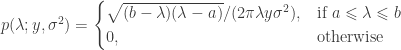
, and  is the Gaussian filter, defined as a function of the geodesic distance between points.
 are known and organised into a distance matrix
  , the filter can take the form of a matrix of the same size,
  , with the values at each row scaled so as to add up to unity, and the same smoothing can proceed as a simple matrix multiplication:
 , truncated at a distance
  from the filter center, in a sphere of radius
  , the number of non-zero elements in
 . Even using sparse matrices, this may require a large amount of memory space. For practical purposes, a filter with width
  = 2), for application in a sphere with 100 mm made by 7 subdivisions of an icosahedron, still comfortably in a computer with 16GB of RAM. Wider filters may require more memory to run.