
Pedigree-based analyses allow investigation of genetic and environmental influences on anatomy, physiology, and behaviour.
Methods based on components of variance have been used extensively to assess genetic influences and identify loci associated with various traits quantifying aspects of anatomy, physiology, and behaviour, in both normal and pathological conditions. In an earlier post, indices of genetic resemblance between relatives were presented, and in the last post, the kinship matrix was defined. In this post, these topics are used to present a basic model that allows partitioning of the phenotypic variance into sources of variation that can be ascribed to genetic, environmental, and other factors.
A simple model
Consider the model:

where, for  subjects,
  traits,
  covariates and
  variance components,
  are the observed trait values for each subject,
  is a matrix of covariates,
  is a matrix of unknown covariates’ weights, and
  are the residuals after the covariates have been taken into account.
The elements of each column  of
of  are assumed to follow a multivariate normal distribution
  , where
  is the between-subject covariance matrix. The elements of each row
  of are assumed to follow a normal distribution
  , where
  is the between-trait covariance matrix. Both and are seen as the sum of variance components, i.e.
  and
and  . For a discussion on these equalities, see Eisenhart (1947) [see references at the end].
An equivalent model
The same model can be written in an alternative way. Let  be the stacked vector of traits,
  is the matrix of covariates,
  the vector with the covariates’ weights,
  the residuals after the covariates have been taken into account, and
  represent the Kronecker product. The model can then be written as:

The stacked residuals  is assumed to follow a multivariate normal distribution
  , where
  can be seen as the sum of variance components:

The here is the same as in Almasy and Blangero (1998).  can be modelled as correlation matrices. The associated scalars are absorbed into the (to be estimated)
  . is the phenotypic covariance matrix between the residuals of the traits:
![\mathbf{R} = \left[ \begin{array}{ccc} \mathsf{Var}(\upsilon_1) & \cdots & \mathsf{Cov}(\upsilon_1,\upsilon_T) \\ \vdots & \ddots & \vdots \\ \mathsf{Cov}(\upsilon_T,\upsilon_1) & \cdots & \mathsf{Var}(\upsilon_T) \end{array}\right]](https://s0.wp.com/latex.php?latex=%5Cmathbf%7BR%7D+%3D+%5Cleft%5B+%5Cbegin%7Barray%7D%7Bccc%7D+%5Cmathsf%7BVar%7D%28%5Cupsilon_1%29+%26+%5Ccdots+%26+%5Cmathsf%7BCov%7D%28%5Cupsilon_1%2C%5Cupsilon_T%29+%5C%5C+%5Cvdots+%26+%5Cddots+%26+%5Cvdots+%5C%5C+%5Cmathsf%7BCov%7D%28%5Cupsilon_T%2C%5Cupsilon_1%29+%26+%5Ccdots+%26+%5Cmathsf%7BVar%7D%28%5Cupsilon_T%29+%5Cend%7Barray%7D%5Cright%5D&bg=ffffff&fg=333333&s=0&c=20201002)
whereas each are the share of these covariances attributable to the  -th component:
![\mathbf{R}_k = \left[ \begin{array}{ccccc} \mathsf{Var}_k(\upsilon_1) & \cdots & \mathsf{Cov}_k(\upsilon_1,\upsilon_T) \\ \vdots & \ddots & \vdots \\ \mathsf{Cov}_k(\upsilon_T,\upsilon_1) & \cdots & \mathsf{Var}_k(\upsilon_T) \end{array}\right]](https://s0.wp.com/latex.php?latex=%5Cmathbf%7BR%7D_k+%3D+%5Cleft%5B+%5Cbegin%7Barray%7D%7Bccccc%7D+%5Cmathsf%7BVar%7D_k%28%5Cupsilon_1%29+%26+%5Ccdots+%26+%5Cmathsf%7BCov%7D_k%28%5Cupsilon_1%2C%5Cupsilon_T%29+%5C%5C+%5Cvdots+%26+%5Cddots+%26+%5Cvdots+%5C%5C+%5Cmathsf%7BCov%7D_k%28%5Cupsilon_T%2C%5Cupsilon_1%29+%26+%5Ccdots+%26+%5Cmathsf%7BVar%7D_k%28%5Cupsilon_T%29+%5Cend%7Barray%7D%5Cright%5D&bg=ffffff&fg=333333&s=0&c=20201002)
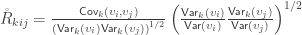
can be converted to a between-trait phenotypic correlation matrix  as:
as:
![\mathbf{\mathring{R}} = \left[ \begin{array}{ccc} \frac{\mathsf{Var}(\upsilon_1)}{\mathsf{Var}(\upsilon_1)} & \cdots & \frac{\mathsf{Cov}(\upsilon_1,\upsilon_T)}{\left(\mathsf{Var}(\upsilon_1)\mathsf{Var}(\upsilon_T)\right)^{1/2}} \\ \vdots & \ddots & \vdots \\ \frac{\mathsf{Cov}(\upsilon_1,\upsilon_T)}{\left(\mathsf{Var}(\upsilon_1)\mathsf{Var}(\upsilon_T)\right)^{1/2}} & \cdots & \frac{\mathsf{Var}(\upsilon_T)}{\mathsf{Var}(\upsilon_T)} \end{array}\right]](https://s0.wp.com/latex.php?latex=%5Cmathbf%7B%5Cmathring%7BR%7D%7D+%3D+%5Cleft%5B+%5Cbegin%7Barray%7D%7Bccc%7D+%5Cfrac%7B%5Cmathsf%7BVar%7D%28%5Cupsilon_1%29%7D%7B%5Cmathsf%7BVar%7D%28%5Cupsilon_1%29%7D+%26+%5Ccdots+%26+%5Cfrac%7B%5Cmathsf%7BCov%7D%28%5Cupsilon_1%2C%5Cupsilon_T%29%7D%7B%5Cleft%28%5Cmathsf%7BVar%7D%28%5Cupsilon_1%29%5Cmathsf%7BVar%7D%28%5Cupsilon_T%29%5Cright%29%5E%7B1%2F2%7D%7D+%5C%5C+%5Cvdots+%26+%5Cddots+%26+%5Cvdots+%5C%5C+%5Cfrac%7B%5Cmathsf%7BCov%7D%28%5Cupsilon_1%2C%5Cupsilon_T%29%7D%7B%5Cleft%28%5Cmathsf%7BVar%7D%28%5Cupsilon_1%29%5Cmathsf%7BVar%7D%28%5Cupsilon_T%29%5Cright%29%5E%7B1%2F2%7D%7D+%26+%5Ccdots+%26+%5Cfrac%7B%5Cmathsf%7BVar%7D%28%5Cupsilon_T%29%7D%7B%5Cmathsf%7BVar%7D%28%5Cupsilon_T%29%7D+%5Cend%7Barray%7D%5Cright%5D&bg=ffffff&fg=333333&s=0&c=20201002)
The above phenotypic correlation matrix has unit diagonal and can still be fractioned into their components:
![\mathbf{\mathring{R}}_k = \left[ \begin{array}{ccc} \frac{\mathsf{Var}_k(\upsilon_1)}{\mathsf{Var}(\upsilon_1)} & \cdots & \frac{\mathsf{Cov}_k(\upsilon_1,\upsilon_T)}{\left(\mathsf{Var}(\upsilon_1)\mathsf{Var}(\upsilon_T)\right)^{1/2}} \\ \vdots & \ddots & \vdots \\ \frac{\mathsf{Cov}_k(\upsilon_T,\upsilon_1)}{\left(\mathsf{Var}(\upsilon_T)\mathsf{Var}(\upsilon_1)\right)^{1/2}} & \cdots & \frac{\mathsf{Var}_k(\upsilon_T)}{\mathsf{Var}(\upsilon_T)} \end{array}\right]](https://s0.wp.com/latex.php?latex=%5Cmathbf%7B%5Cmathring%7BR%7D%7D_k+%3D+%5Cleft%5B+%5Cbegin%7Barray%7D%7Bccc%7D+%5Cfrac%7B%5Cmathsf%7BVar%7D_k%28%5Cupsilon_1%29%7D%7B%5Cmathsf%7BVar%7D%28%5Cupsilon_1%29%7D+%26+%5Ccdots+%26+%5Cfrac%7B%5Cmathsf%7BCov%7D_k%28%5Cupsilon_1%2C%5Cupsilon_T%29%7D%7B%5Cleft%28%5Cmathsf%7BVar%7D%28%5Cupsilon_1%29%5Cmathsf%7BVar%7D%28%5Cupsilon_T%29%5Cright%29%5E%7B1%2F2%7D%7D+%5C%5C+%5Cvdots+%26+%5Cddots+%26+%5Cvdots+%5C%5C+%5Cfrac%7B%5Cmathsf%7BCov%7D_k%28%5Cupsilon_T%2C%5Cupsilon_1%29%7D%7B%5Cleft%28%5Cmathsf%7BVar%7D%28%5Cupsilon_T%29%5Cmathsf%7BVar%7D%28%5Cupsilon_1%29%5Cright%29%5E%7B1%2F2%7D%7D+%26+%5Ccdots+%26+%5Cfrac%7B%5Cmathsf%7BVar%7D_k%28%5Cupsilon_T%29%7D%7B%5Cmathsf%7BVar%7D%28%5Cupsilon_T%29%7D+%5Cend%7Barray%7D%5Cright%5D&bg=ffffff&fg=333333&s=0&c=20201002)
The relationship  holds. The diagonal elements of
  may receive particular names, e.g., heritability, environmentability, dominance effects, shared enviromental effects, etc., depending on what is modelled in the corresponding . However, the off-diagonal elements of are not the
  that correspond, e.g. to the genetic or environmental correlation. These off-diagonal elements are instead the signed
  when
when  , or their
  -equivalent for other variance components (see below). In this particular case, they can also be called “bivariate heritabilities” (Falconer and MacKay, 1996). A matrix
  that contains these correlations , which are the fraction of the variance attributable to the -th component that is shared between pairs of traits is given by:
![\mathbf{\breve{R}}_k = \left[ \begin{array}{ccc} \frac{\mathsf{Var}_k(\upsilon_1)}{\mathsf{Var}_k(\upsilon_1)} & \cdots & \frac{\mathsf{Cov}_k(\upsilon_1,\upsilon_T)}{\left(\mathsf{Var}_k(\upsilon_1)\mathsf{Var}_k(\upsilon_T)\right)^{1/2}} \\ \vdots & \ddots & \vdots \\ \frac{\mathsf{Cov}_k(\upsilon_T,\upsilon_1)}{\left(\mathsf{Var}_k(\upsilon_T)\mathsf{Var}_k(\upsilon_1)\right)^{1/2}} & \cdots & \frac{\mathsf{Var}_k(\upsilon_T)}{\mathsf{Var}_k(\upsilon_T)} \end{array}\right]](https://s0.wp.com/latex.php?latex=%5Cmathbf%7B%5Cbreve%7BR%7D%7D_k+%3D+%5Cleft%5B+%5Cbegin%7Barray%7D%7Bccc%7D+%5Cfrac%7B%5Cmathsf%7BVar%7D_k%28%5Cupsilon_1%29%7D%7B%5Cmathsf%7BVar%7D_k%28%5Cupsilon_1%29%7D+%26+%5Ccdots+%26+%5Cfrac%7B%5Cmathsf%7BCov%7D_k%28%5Cupsilon_1%2C%5Cupsilon_T%29%7D%7B%5Cleft%28%5Cmathsf%7BVar%7D_k%28%5Cupsilon_1%29%5Cmathsf%7BVar%7D_k%28%5Cupsilon_T%29%5Cright%29%5E%7B1%2F2%7D%7D+%5C%5C+%5Cvdots+%26+%5Cddots+%26+%5Cvdots+%5C%5C+%5Cfrac%7B%5Cmathsf%7BCov%7D_k%28%5Cupsilon_T%2C%5Cupsilon_1%29%7D%7B%5Cleft%28%5Cmathsf%7BVar%7D_k%28%5Cupsilon_T%29%5Cmathsf%7BVar%7D_k%28%5Cupsilon_1%29%5Cright%29%5E%7B1%2F2%7D%7D+%26+%5Ccdots+%26+%5Cfrac%7B%5Cmathsf%7BVar%7D_k%28%5Cupsilon_T%29%7D%7B%5Cmathsf%7BVar%7D_k%28%5Cupsilon_T%29%7D+%5Cend%7Barray%7D%5Cright%5D&bg=ffffff&fg=333333&s=0&c=20201002)
As for the phenotypic correlation matrix, each has unit diagonal.
The most common case
A particular case is when  , the coefficient of familial relationship between subjects, and
  . In this case, the diagonal elements of
  represent the heritability (
 ) for each trait . The diagonal of
  contains
  , the environmentability. The off-diagonal elements of contain the signed (see below). The genetic correlations,
  are the off-diagonal elements of
  , whereas the off-diagonal elements of
  are
are  , the environmental correlations between traits. In this particular case, the components of , i.e., are equivalent to
  and
and  covariance matrices as in Almasy et al (1997).
Relationship with the ERV
To see how the off-diagonal elements of are the signed Endophenotypic Ranking Values for each of the -th variance component, (Glahn et al, 2011), note that for a pair of traits  and
and  :
:

Multiplying both numerator and denominator by  and rearranging the terms gives:
When  , the above reduces to
  , which is the signed version of
  when is the genetic component.
Positive-definiteness
and are covariance matrices and so, are positive-definite, whereas the correlation matrices , and are positive-semidefinite. A hybrid matrix that does not have to be positive-definite or semidefinite is:

where  is a matrix of ones,
  is the identity, both of size
  , and
, and  is the Hadamard product. An example of such matrix of practical use is to show concisely the heritabilities for each trait in the diagonal and the genetic correlations in the off-diagonal.
Cauchy-Schwarz
Algorithmic advantages can be obtained from the positive-definiteness of . The Cauchy–Schwarz theorem (Cauchy, 1821; Schwarz, 1888) states that:

Hence, the bounds for the off-diagonal elements can be known from the diagonal elements, which, by their turn, are estimated in a simpler, univariate model.

The Cauchy-Schwarz inequality imposes limits on the off-diagonal values of the matrix that contains the genetic covariances (or bivariate heritabilities).
Parameter estimation
Under the multivariate normal assumption, the parameters can be estimated maximising the following loglikelihood function:

where  is the number of observations on the stacked vector
  . Unbiased estimates for
  , although inefficient and inappropriate for hypothesis testing, can be obtained with ordinary least squares (OLS).
Parametric inference
Hypothesis testing can be performed with the likelihood ratio test (LRT), i.e., the test statistic is produced by subtracting from the loglikelihood of the model in which all the parameters are free to vary ( ), the loglikelihood of a model in which the parameters being tested are constrained to zero, the null model (
 ). The statistic is given by
  (Wilks, 1938), which here is asymptotically distributed as a 50:50 mixture of a
  and
and  distributions, where df is the number of parameters being tested and free to vary in the unconstrained model (Self and Liang, 1987). From this distribution the p-values can be obtained.
References
- Almasy L, Blangero J. Multipoint quantitative-trait linkage analysis in general pedigrees. Am J Hum Genet. 1998 May;62(5):1198–211.
- Almasy L, Dyer TD, Blangero J. Bivariate quantitative trait linkage analysis: pleiotropy versus co-incident linkages. Genet Epidemiol. 1997 Jan;14(6):953–8.
- Cauchy, A-L. Œuvres Completes D’Augustin Cauchy (published in 1882). Vol. XV. Gauthier-Villars et Fils, Paris, 1821.
- Eisenhart C. The assumptions underlying the analysis of variance. Biometrics. 1947;3(1):1–21.
- Falconer DS, Mackay TFC. Introduction to Quantitative Genetics. Addison Wesley Longman, Harlow, Essex, UK, 1996.
- Glahn DC, Curran JE, Winkler AM, Carless MA, Kent JW, Charlesworth JC, et al. High dimensional endophenotype ranking in the search for major depression risk genes. Biol Psychiatry. 2012 Jan 1;71(1):6–14.
- Schwarz HA. Über ein Flächen kleinsten Flächeninhalts betreffendes Problem der Variationsrechnung. Acta Societatis Scientiarum Fennicæ XV, 319–332, 1888.
- Self SG, Liang KY. Asymptotic properties of maximum likelihood estimators and likelihood ratio tests under nonstandard conditions. J Am Stat Assoc. 1987;82(398):605–10.
- Wilks SS. The Large-Sample Distribution of the Likelihood Ratio for Testing Composite Hypotheses. Ann Math Stat. 1938;9(1):60–2.
The photograph at the top (elephants) is by Anja Osenberg and was generously released into public domain.


 , is probably the most interesting. It gives a probabilistic estimate that a random gene from a given subject
  subjects, these probabilities can be assembled in a
  matrix termed kinship matrix, usually represented as
  , that has elements
  , and that can be used to model the covariance between individuals in quantitative genetics.
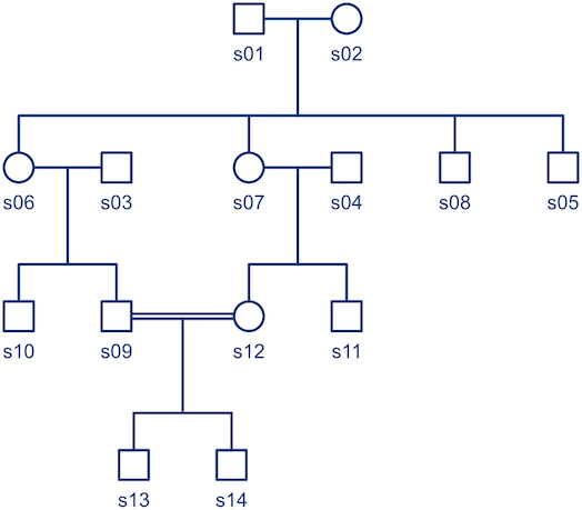
 ), is:
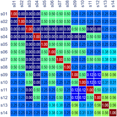

 . Each individual has two copies, one from paternal, another from maternal origin; these can be indicated as
  and
and  for individual
 , a respective probability
  can be assigned; these are called coefficients of identity by descent. These probabilities can be calculated at every generation following very elementary rules. For most problems, however, the distinction between paternal and maternal origin of a gene is irrelevant, and some of the above states are equivalent to others. If these are condensed, we can retain 9 distinct ways, shown in the figure below:
 , a respective probability
  can be assigned; these are called condensed coefficients of identity by descent, and relate to the former as:


 ,
,  and
and  correspond to his coefficients
  ,
,  and
and  .
.
 is the kinship of a subject with himself. Two genes taken from the same individual can either be the same gene (probability
  of being the same) or be the genes inherited from father and mother, in which case the probability is given by the coefficient of kinship between the parents. In other words,
  . If both parents are unrelated,
  , such that the kinship of a subject with himself is
  .
. (see below about the coefficient of inbreeding,
  ). Thus, if there are
  generations between
  generations between
  . If
. If 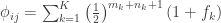
 , and used to model the covariance between subjects as
  (
( can be computed from the coefficients of identity:


 is the transformed value for observation
  is the
  is the ordinary rank of the
 is a constant and the remaining variables are as above. The value of
  , Tukey (1962) suggests
  , Bliss (1967) suggests
  and, as just decribed, Van der Waerden suggests
  .
.