Retrospective motion correction for structural MRI

Posted on 17.May.2012 by A. M. Winkler

Good quality results can only be obtained with good quality images. To obtain images with good SNR and high resolution, long scan times are often necessary. However, with longer acquisition, the subjects are more likely to move. Rather than acquire a very long sequence, that often can last up to 40 minutes, the acquisition can be broken into many shorter scans, each with lower SNR. These are coregistered, effectively reducing the effect of undesired movement, and averaged, for increase of the SNR (Kochunov et al, 2006).

The last image in the second row is the average of all the other seven, after retrospective motion correction has been applied.

The results above are typical. Each pixel above corresponds to a true voxel, with no interpolation. Therefore, to see in more detail, simply download the image above and use an image viewer (e.g. gwenview or eog) to zoom.

The method is termed retrospective to discern it from prospective motion correction methods, such as those available for BOLD-sensitive EPI acquisitions (e.g. Siemens 3D PACE).

Since the images belong to the same subject and typically the movement is of only a few degrees or milimeters, the affine matrices for these corrections should have a diagonal with values very close to 1 and very close to zero off the diagonal. Here is one example:

0.999995    -0.00020007  -0.0030414    0.106906
0.000188555  0.999993    -0.00378601   0.100499
0.00304214   0.00378542   0.999988    -0.204133
0            0            0            1

As usual, the improvement in the SNR is given by a factor of $\sqrt{n}$ , where $n$ is the number of images averaged.

Download

A script to apply the method is available here: stereomc. Just download and make it executable. Call it without arguments to obtain usage information.

Requirements

FSL tools must be installed and properly configured.

Reference

Kochunov P, Lancaster JL, Glahn DC, Purdy D, Laird AR, Gao F, Fox P. Retrospective motion correction protocol for high-resolution anatomical MRI. Hum Brain Mapp. 2006 Dec;27(12):957-62.

The logic of the Fisher method to combine P-values

Posted on 11.May.2012 by A. M. Winkler

Consider a set of $k$ independent tests, each of these to test a certain null hypothesis $\mathcal{H}_{0|i}$ , $i=\{1, 2, \ldots, k\}$ . For each test, a significance level $P_{i}$ , i.e., a p-value, is obtained. All these p-values can be combined into a joint test whether there is a global effect, i.e., if a global null hypothesis $\mathcal{H}_0$ can be rejected.

There are a number of ways to combine these independent, partial tests. The Fisher method is one of these, and is perhaps the most famous and most widely used. The test was presented in Fisher’s now classical book, Statistical Methods for Research Workers, and was described rather succinctly:

When a number of quite independent tests of significance have been made, it sometimes happens that although few or none can be claimed individually as significant, yet the aggregate gives an impression that the probabilities are on the whole lower than would often have been obtained by chance. It is sometimes desired, taking account only of these probabilities, and not of the detailed composition of the data from which they are derived, which may be of very different kinds, to obtain a single test of the significance of the aggregate, based on the product of the probabilities individually observed.
The circumstance that the sum of a number of values of $\chi^{2}$ is itself distributed in the $\chi^{2}$ distribution with the appropriate number of degrees of freedom, may be made the basis of such a test. For in the particular case when $n=2$ , the natural logarithm of the probability is equal to $\frac{1}{2}\chi^{2}$ . If therefore we take the natural logarithm of a probability, change its sign and double it, we have the equivalent value of $\chi^{2}$ for 2 degrees of freedom. Any number of such values may be added together, to give a composite test, using the Table of $\chi^{2}$ to examine the significance of the result. — Fisher, 1932.

The test is based on the fact that the probability of rejecting the global null hypothesis is related to intersection of the probabilities of each individual test, $\prod_{i} P_{i}$ . However, $\prod_{i} P_{i}$ is not uniformly distributed, even if the null is true for all partial tests, and cannot be used itself as the joint significance level for the global test. To remediate this fact, some interesting properties and relationships among distributions of random variables were exploited by Fisher and embodied in the succinct excerpt above. These properties are discussed below.

The logarithm of uniform is exponential

The cumulative distribution function (cdf) of an exponential distribution is:

$F(x)=1- e^{-\lambda x}$

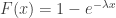
where $\lambda$ is the rate parameter, the only parameter of this distribution. The inverse cdf is, therefore, given by:

$x = -\dfrac{1}{\lambda}\ln(1-F(x))$

If $P$ is a random variable uniformly distributed in the interval $[0, 1]$ , so is $1-P$ , and it is immaterial to differ between them. As a consequence, the previous equation can be equivalently written as:

$x = -\dfrac{1}{\lambda}\ln(P)$

where $P \sim \mathcal{U}(0,1)$ , which highlights the fact that the negative of the natural logarithm of a random variable distributed uniformly between 0 and 1 follows an exponential distribution with rate parameter $\lambda=1$ .

An exponential with rate 1/2 is chi-squared

The cdf of a chi-squared distribution with $\nu$ degrees of freedom, i.e. $\chi^{2}_{\nu}$ , is given by:

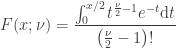
$F(x; \nu) = \dfrac{\int_{0}^{x/2} t^{\frac{\nu}{2}-1}e^{-t}{\rm d}t}{\left(\frac{\nu}{2}-1\right)!}$

If $\nu=2$ , and solving the integral we have:

$F(x; \nu=2) = \dfrac{\int_{0}^{x/2} t^{\frac{2}{2}-1}e^{-t}{\rm d}t}{\left(\frac{2}{2}-1\right)!} = \int_{0}^{x/2} e^{-t}{\rm d}t = 1-e^{-x/2}$

In other words, a $\chi^{2}$ distribution with $\nu=2$ is equivalent to an exponential distribution with rate parameter $\lambda=1/2$ .

The sum of chi-squared is also chi-squared

The moment-generating function (mgf) of a sum of independent variables is the product of the mgfs of the respective variables. The mgf of a $\chi^{2}_{\nu}$ is:

$M(t) = (1-2t)^{-\nu/2}$

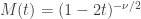
The mgf of the sum of $k$ independent variables that follow each a $\chi^{2}_{2}$ distribution is then given by:

$M_{\text{sum}}(t) = \prod_{i=1}^{k} (1-2t)^{-2/2} = (1-2t)^{-k}$

which also defines a $\chi^{2}$ distribution, however with degrees of freedom $\nu=2k$ .

Assembling the pieces

With these facts in mind, how to transform the product $\prod_{i} P_{i}$ into a p-value that is uniformly distributed when the global null is true? The product can be converted into a sum by taking the logarithm. And as shown above, the logarithm of uniformly distributed variables follows an exponential distribution with rate parameter $\lambda=1$ . Multiplication of each $\ln(P_{i})$ by 2 changes the rate parameter to $\lambda=1/2$ and makes this distribution equivalent to a $\chi^{2}$ distribution with degrees of freedom $\nu=2$ . The sum of $k$ of these logarithms also follow a $\chi^2$ distribution, now with $\nu=2k$ degrees of freedom, i.e., $\chi^{2}_{2k}$ .

The statistic for the Fisher method is, therefore, computed as:

$X = -2 \sum_{i=1}^{k} \ln(P_{i})$

with $X$ following a $\chi^{2}_{2k}$ distribution, from which a p-value for the global hypothesis can be easily obtained.

Reference

The details above are not in the book, presumably omitted by Fisher as the knowledge of these derivation details would be of little practical use. Nonetheless, the reference for the book is:

Fisher, R. A., 1932. Statistical Methods for Research Workers, 4th Edition. Oliver and Boyd, Edinburgh.

Importing FreeSurfer subcortical structures into Blender

Posted on 08.May.2012 by A. M. Winkler

In a previous article, a method to import cortical meshes from FreeSurfer into Blender and other CG applications was presented. Here it is complemented with a method to import the subcortical structures. These structures are segmented as part of FreeSurfer subcortical stream, and are stored in a volume-based representation. In order to import into Blender, first it is necessary to generate surfaces, then convert to Wavefront OBJ, and finally, do the import. Below is an example of how the output looks like.

An example of a subcortical meshes generated from FreeSurfer subcortical segmentations imported into Blender.

Generating the surfaces for subcortical structures

The surfaces can be generated using FreeSurfer’s own tools. The script aseg2srf automates the task. Suppose you would like to create meshes for all subcortical structures of the subjects named “capitu”, “bentinho” and “ezequiel”. Simply run:

aseg2srf -s "capitu bentinho ezequiel"

The outputs are saved in a directory called ascii, inside each subject’s directory. The script requires that FreeSurfer is installed and working properly, and that the environmental variable ${SUBJECTS_DIR} has been set to point to the location where the subjects are. It is also necessary to have writing permissions to this directory, so that the surfaces can be saved.

If there are many subjects, provide a list from a text file, with one subject per line:

aseg2srf -s list.txt

To make surfaces for just some structures, provide their label numbers with the -l option. For the hippocampus, for instance, the labels are 17 and 53 for left and right respectively:

aseg2srf -s "capitu bentinho ezequiel" -l "17 53"

The script has also a -d option, for debugging, which allows to keep temporary files used during the mesh generation.

List of labels

Below is a list of the label codes for the major structures. A more comprehensive list is in the aseg.stats file, inside the stats directory for each subject, or in the FreeSurferColorLUT.txt file (in the FreeSurfer directory).

Left lateral ventricle	4
Left inferior part of the lateral ventricle	5
Left cerebellum white matter	7
Left cerebellum cortex	8
Left thalamus	10
Left caudate	11
Left putamen	12
Left pallidum	13
Left hippocampus	17
Left amygdala	18
CSF	24
Left accumbens	26
Left ventral diencephalon	28
Left choroid plexus	31
Right lateral ventricle	43
Right inferior part of the lateral ventricle	44
Right cerebellum white matter	46
Right cerebellum cortex	47
Right thalamus	49
Right caudate	50
Right putamen	51
Right pallidum	52
Right hippocampus	53
Right amygdala	54
Right accumbens	58
Right ventral diencephalon	60
Right choroid plexus	63
Corpus callosum, posterior part	251
Corpus callosum, middle posterior part	252
Corpus callosum, central part	253
Corpus callosum, middle anterior part	254
Corpus callosum, anterior part	255
3rd ventricle	14
4th ventricle	15
5th ventricle (CSF sometimes found in the septum pellucidum)	72
Brain stem	16

Conversion to Wavefront OBJ

Once the meshes have been generated, the process of conversion into a format that can be read by CG software is the same as described previously here.

Download

The script is available here: aseg2srf.

Requirements

FreeSurfer must be installed and working properly. The environmental variable ${SUBJECTS_DIR} must point to the directory where the data for each subject is located. It is also assumed that recon-all has been run successfully.

Importing FreeSurfer cortical meshes into Blender

Posted on 08.May.2012 by A. M. Winkler

Computer graphics (CG) applications, such as Blender, Maya or 3D Studio, doesn’t come with filters that allow to directly import or export FreeSurfer meshes. To import brain surfaces to these applications, converting first to an intermediate file format solves the problem. Below is an example of a brain imported into Blender.

An example of a brain mesh from FreeSurfer imported into Blender after conversion to Wavefront OBJ.

The mris_convert, from FreeSurfer, allows conversion to stereolithography format (STL). However, not all CG applications read natively from STL files. Moreover, other formats, such as Wavefront OBJ and Stanford PLY have simpler structure — yet allowing features that will be discussed here in forthcoming articles.

Conversion from FreeSurfer to Wavefront OBJ

A simple procedure to convert a FreeSurfer surface to Wavefront OBJ (ASCII) is:

1) Use mris_convert to convert from FreeSurfer binary to ASCII:

mris_convert lh.pial lh.pial.asc

2) A suggestion is to rename the .asc file to .srf, to differentiate it from other files that also have .asc extension and have a different internal structure.

mv lh.pial.asc lh.pial.srf

3) Use the script srf2obj to convert from .srf to .asc:

srf2obj lh.pial.srf > lh.pial.obj

The symbol “>” is necessary so that the output from srf2obj is redirected to a new file.

Conversion from Wavefront OBJ to FreeSurfer

To convert back to FreeSurfer, a similar strategy is used.

1) Use the script obj2srf to generate new .srf files (here directly named as .asc, as expected by mris_convert)

obj2srf lh.pial.obj > lh.pial.asc

2) Use mris_convert:

mris_convert lh.pial.asc lh.pial

Download

Both scripts are available here: srf2obj and obj2srf. Right-click and save, then make them executable.

Requirements

The scripts use gawk as the interpreter, and expects to find it on its usual location (/bin/gawk). If in your system gawk is installed elsewhere, modify the first line accordingly.

If you don’t have gawk, you can get it from the repository of your Linux distribution. For Mac, gawk is available in MacPorts and Fink. Alternatively, you may replace gawk with awk itself, nawk, or any other awk implementation that works.