Braindering with ASCII files

Posted on 25.September.2011 by A. M. Winkler

Binary file formats are faster to read and occupy less space for storage. However, when developing tools or when analysing data using non-standard methods, ascii files are easier to treat, and allow certain errors to be spotted immediately. Working with ascii files offer a number of advantages in these circumstances: the content of the files are human readable, meaning that there is no need for any special program other than perhaps a simple text editor, and can be manipulated easily with tools as sed or awk. It should be noted though, that while binary files require attention with respect to endianess and need some metadata to be correctly read, ascii need proper attention to end-of-line characters, that vary according to the operating system.

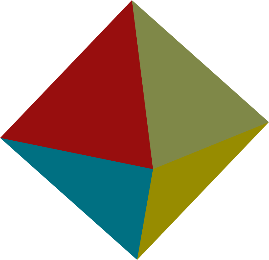
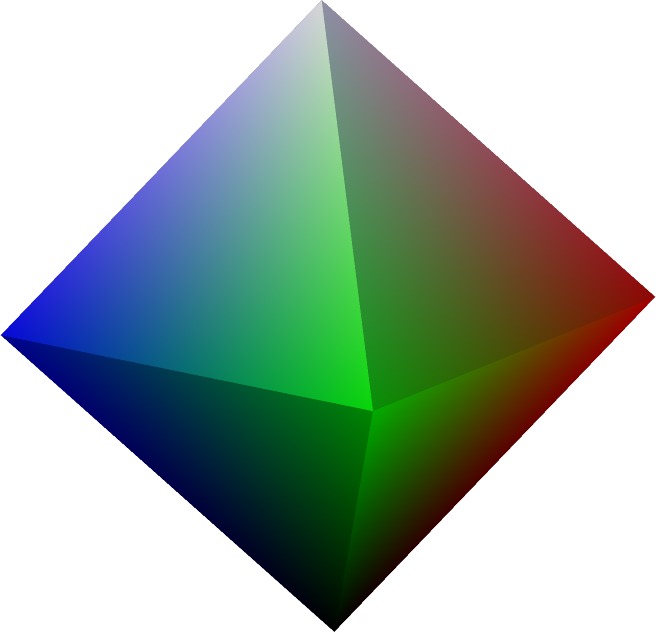
In articles to be posted soon I hope to share some tools to analyse and visualise brain imaging data. To use these tools, the files must be in ascii format. Each of these formats is discussed below and an example is given for a simple octahedron.

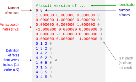
FreeSurfer surface (.asc | suggested: .srf)

FreeSurfer natively saves its surface files in binary form. The command mris_convert allows conversion to ascii format. The file extension is *.asc. This extension, however, is ambiguous with the curvature format (see below), reason for which a recommendation is to rename from *.asc to *.srf immediately after conversion.

The *.asc/*.srf format has a structure as described below. This format does not allow storing normals, colors, materials, multiple objects or textures. Just simple geometry.

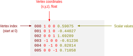
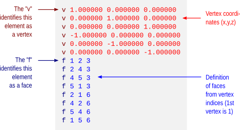
FreeSurfer curvature (.asc | suggested: .dpv)

A curvature file contains a scalar value assigned to each vertex. This file format does not store the geometry of the surface and, in binary form, a curvature file simply contains one scalar per vertex. In ascii format, the vertex coordinates are also saved, but not how these vertices relate to define faces and the overall geometry.

Like with the FreeSurfer surface files, curvature files in ascii format also have the extension *.asc. To avoid confusion, it is suggested to rename from *.asc to *.dpv (data-per-vertex) immediately after conversion.

Facewise data (*.dpf)

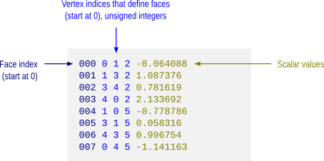
This is not a native format from FreeSurfer, but a modification over the ascii curvature file described above. The file stores a scalar value per face, i.e. data-per-face (dpf) and, instead of saving vertex coordinates as with the *.dpv files, here the vertex indices that define the faces are saved. It is done like so because if both *.dpv and *.dpf files are present for a given geometric object, the object can be reconstructed with very little manipulation using simply awk. Currently there is no binary equivalent format.

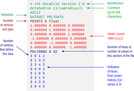
VTK polygonal data (*.vtk)

A number of file formats have been developed over the years for use with the Visualization Toolkit (vtk). Some of these formats are now considered as “legacy” and are being phased out in favour of xml formats. Despite this, they are still used by a number of applications, such as fsl/first. The octahedron above in vtk polygonal data (polydata) format would have a structure as depicted below.

Wavefront Object (*.obj)

Wavefront Object files have a very simple structure, yet are powerful to allow definition of textures, normals and different materials. The format is supported by a variety of different graphic applications. The octahedron above would have a file structure as shown below.

The example does not show colors. However, it is possible to assign a material to each face, and materials contain their own color. These materials are typically stored in a separate file, a Materials Library, with extension *.mtl. An example for the same octahedron, both the object file and its associated materials library, is here: octa-color.obj and octa-color.mtl.

Many computer graphics software, however, limit the number of colors per object to a relatively small number, as 16 or 32. Blender, however, allows 32767 colors per object, a comfortable space for visualization of complex images, such as brain maps.

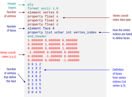
Stanford Polygon (*.ply)

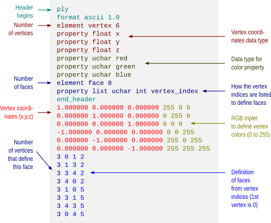
The Stanford Polygon file allows not only the geometry to be stored, but also allow colours, transparency, confidence intervals and other properties to be assigned at each vertex. Again, the octahedron would have a file structure as:

This format also allows color attributes to be assigned to each vertex, as shown below.

The resulting object would then look like:

Batch conversion

Conversion between FreeSurfer formats can be done using mris_convert. A script to batch convert all FreeSurfer surface and curvature files from binary format to ascii is available here: subj2ascii. Before running, make sure FreeSurfer is correctly configured, that the variable SUBJECTS_DIR has been correctly set, and that you have writing permissions to this directory. Execute the script with no arguments to get usage information. The outputs (*.srf and *.dpv) are saved in a directory called ascii inside the directory of the subject. For many subjects, use a for-loop in the shell.

For more information

A description of the FreeSurfer file formats is available here.
A description of the different vtk (legacy and current) is available here.
Specification of the Wavefront obj format is here. Material library files are described here.
A description of the Stanford ply format is here.

Update — 28.May.2012: A script to convert from FreeSurfer .asc/.srf to .obj is here.
Update — 26.Jul.2013: This post was just updated to include examples of color formats.

Quickly inspect FreeSurfer cortical surfaces

Posted on 10.September.2011 by A. M. Winkler

To quickly inspect the surface reconstruction and parcellations produced by the cortical stream of FreeSurfer, rather than laboriously open each hemisphere at a time in tksurfer, an easier solution is to run a script that captures images, organise and present them all in a single html page that can be seen in any browser.

Before you start

Before you start, make sure you have:

FreeSurfer, any version released in the last 2 years. The procedure has been tested up to version 5.1.0.
ImageMagick, any recent version. For most Linux, ImageMagick can be installed directly from the distro’s repository. For Mac, it can be obtained with MacPorts or Fink.
The scripts takeshots, makehtml, shots_tksurfer.tcl, and shots_tkmedit.tcl. Put all these scripts into the same directory and make takeshots and makehtml executable.

Capturing the images

Make sure recon-all finished for all your subjects. If there are no results, obviously there won’t be anything to inspect.
Make sure the variable SUBJECTS_DIR is correctly set, pointing to the directory that contains the subjects, and that you have writing permissions to this directory.
Prepare a text file containing a list of subjects, one per line, like this:
subj001 subj002 ... subjNN
Run the takeshots script. A typical usage is like this:
./takeshots -l listsubj.txt -m pial -m inflated -p aparc
The options are:
-l: List of subjects.
-s: Additional subjects not in the list.
-m: Surfaces to inspect (pial, inflated, white, sphere, etc).
-p: Parcellations to inspect (aparc, aparc.a2005s, aparc.a2009s, etc).
This script will create a subdirectory called ‘shots’ inside the directory of each subject, and will store a number of .tif files that are the different views of the cortical surfaces.
Run the makehtml script. A typical usage is like this:
./makehtml -l listsubj.txt -m pial -m inflated -p aparc -d /path/to/html
The options are identical to the previous command, with the addition of the option -d that lets you specify a directory where the html will be created. If this directory doesn’t exist, it will be created.

What you get

Open the file index.html in the directory specified in the previous step. There you’ll see all the surfaces of all the subjects, all in the same page, allowing you to quickly compare and have an idea of how good or bad they are. To see the name of the subject, hover the mouse on the corresponding image. Click on the image to see it larger. An example, using only pial and inflated surfaces, and the aparc parcellation, is here.

False Discovery Rate: Corrected & Adjusted P-values

Posted on 05.September.2011 by A. M. Winkler

Until mid-1990’s, control of the error rate under multiple testing was done, in general, using family-wise error rate (FWER). An example of this kind of correction is the Bonferroni correction. In an influential paper, Benjamini and Hochberg (1995) introduced the concept of false discovery rate (FDR) as a way to allow inference when many tests are being conducted. Differently than FWER, which controls the probability of committing a type I error for any of a family of tests, FDR allows the researcher to tolerate a certain number of tests to be incorrectly discovered. The word rate in the FDR is in fact a misnomer, as the FDR is the proportion of discoveries that are false among all discoveries, i.e., proportion of incorrect rejections among all rejections of the null hypothesis.

Benjamini and Hochberg’s FDR-controlling procedure

Consider testing $N$ hypotheses, $H_{1}, H_{2}, \ldots , H_{N}$ based on their respective p-values, $p_{1}, p_{2}, \ldots , p_{N}$ . Consider that a fraction $q$ of discoveries are allowed (tolerated) to be false. Sort the p-values in ascending order, $p_{(1)} \leq p_{(2)} \leq \ldots \leq p_{(N)}$ and denote $H_{(i)}$ the hypothesis corresponding to $p_{(i)}$ . Let $k$ be the largest $i$ for which $p_{(i)} \leq \frac{i}{N}\frac{q}{c(N)}$ . Then reject all $H_{(i)}$ , $i=1, 2, \ldots , k$ . The constant $c(N)$ is not in the original publication, and appeared in Benjamini and Yekutieli (2001) for cases in which independence cannot be ascertained. The possible choices for the constant are $c(N)=1$ or $c(N)=\sum_{i=1}^{N} 1/i$ . The second is valid in any situation, whereas the first is valid for most situations, particularly where there are no negative correlations among tests. The B&H procedure has found many applications across different fields, including neuroimaging, as introduced by Genovese et al. (2002).

FDR correction

The procedure described above effectively defines a single number, a threshold, that can be used to declare tests as significant or not at the level $q$ . One might, instead, be interested to know, for each original p-value, the minimum $q$ level in which they would still be rejected. To find this out, define $q_{(i)}=\frac{p_{(i)}N}{i}c(N)$ . This formulation, however, has problems, as discussed next.

FDR adjustment

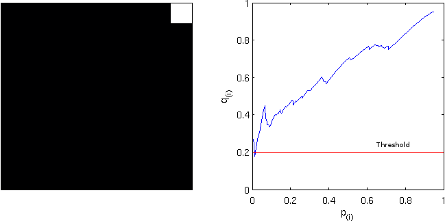
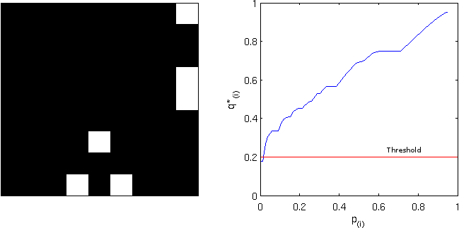
The problem with the FDR-correction is that $q_{(i)}$ is not a monotonic function of $p_{(i)}$ . This means that if someone uses any $q_{(i)}$ to threshold the set of FDR-corrected values, the result is not the same as would be obtained by applying sequentially the B&H procedure for all these corresponding $q$ levels.

To address this concern, Yekutieli and Benjamini (1999) introduced the FDR-adjustment, in which monotonicity is enforced, and which definition is compatible with the original FDR definition. Let $q*_{(i)}$ be the FDR-adjusted value for $p_{(i)}$ . It’s value is the smallest $q_{(k)}, k \geq i$ , where $q_{(k)}$ is the FDR-corrected as defined above. That’s just it!

Example

Consider the image below, on the left, a square of 9×9 pixels containing each some t-statistic with some sparse, low magnitude signal added. On the right are the corresponding p-values, ranging approximately between 0-1:

Statistical maps

Statistic and p-values

colorscale

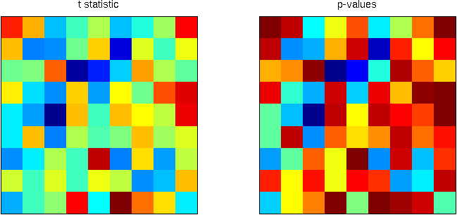
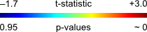
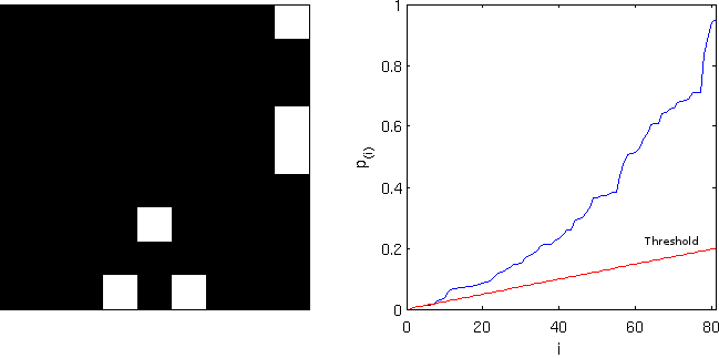
Using the B&H procedure to compute the threshold, with $q=0.20$ , and applying this threshold to the image rejects the null hypothesis in 6 pixels. On the right panel, the red line corresponds to the threshold. All p-values (in blue) below this line are declared significant.

FDR-threshold

FDR-threshold

Computing the FDR-corrected values at each pixel, and thresholding at the same $q=0.20$ , however, does not produce the same results, and just 1 pixel is declared significant. Although conservative, the “correction” is far from the nominal false discovery rate and is not appropriate. Note on the right panel the lack of monotonicity.

FDR-corrected

FDR-corrected

Computing instead the FDR-adjusted values, and thresholding again at $q=0.20$ produces the same results as with the simpler FDR-threshold. The adjustment is, thus, more “correct” than the “corrected”. Observe, on the right panel, the monotonicity enforced.

FDR-adjusted

FDR-adjusted

Implementation

An implementation of the three styles of FDR for Octave/MATLAB is available here: fdr.m
SPM users will find a similar feature in the function spm_P_FDR.m.