Permutation tests in the Human Connectome Project

Posted on 07.December.2015 by A. M. Winkler

Permutation tests are known to be superior to parametric tests: they are based on only few assumptions, essentially that the data are exchangeable, and allow the correction for the multiplicity of tests and the use of various non-standard statistics. The exchangeability assumption allows data to be permuted whenever their joint distribution remains unaltered. Usually this means that each observation needs to be independent from the others.

In many studies, however, there are repeated measurements on the same subjects, which violates exchangeability: clearly, the various measurements obtained from a given subject are not independent from each other. In the Human Connectome Project (HCP) (Van Essen et al, 2012; 2013; see references at the end), subjects are sampled along with their siblings (most of them are twins), such that independence cannot be guaranteed either.

In Winkler et al. (2014), certain structured types of non-independence in brain imaging were addressed through the definition of exchangeability blocks (EBs). Observations within EB can be shuffled freely or, alternatively, the EBs themselves can be shuffled as a whole. This allows various designs that otherwise could not be assessed through permutations.

The same idea can be generalised for blocks that are nested within other blocks, in a multi-level fashion. In the paper Multi-level Block Permutation (Winkler et al., 2015) we presented a method that allows blocks to be shuffled a whole, and inside them, sub-blocks are further allowed to be shuffled, in a recursive process. The method is flexible enough to accommodate permutations, sign-flippings (sometimes also called “wild bootstrap”), and permutations together with sign-flippings.

In particular, this permutation scheme allows the data of the HCP to be analysed via permutations: subjects are allowed to be shuffled with their siblings while keeping the joint distribution intra-sibship maintained. Then each sibship is allowed to be shuffled with others of the same type.

In the paper we show that the error type I is controlled at the nominal level, and the power is just marginally smaller than that would be obtained by permuting freely if free permutation were allowed. The more complex the block structure, the larger the reductions in power, although with large sample sizes, the difference is barely noticeable.

Importantly, simply ignoring family structure in designs as this causes the error rates not to be controlled, with excess false positives, and invalid results. We show in the paper examples of false positives that can arise, even after correction for multiple testing, when testing associations between cortical thickness, cortical area, and measures of body size as height, weight, and body-mass index, all of them highly heritable. Such false positives can be avoided with permutation tests that respect the family structure.

The figure at the top shows how the subjects of the HCP (terminal dots, shown in white colour) can be shuffled or not, while respecting the family structure. Blue dots indicate branches that can be permuted, whereas red dots indicate branches that cannot (see the main paper for details). This diagram includes 232 subjects of an early public release of HCP data. The tree on the left considers dizygotic twins as a category on their own, i.e., that cannot be shuffled with ordinary siblings, whereas the tree on the right considers dizygotic twins as ordinary siblings.

The first applied study using our strategy has just appeared. The method is implemented in the freely available package PALM — Permutation Analysis of Linear Models, and a set of practical steps to use it with actual HCP data is available here.

References

Van Essen DC, Ugurbil K, Auerbach E, Barch D, Behrens TE, Bucholz R, Chang A, Chen L, Corbetta M, Curtiss SW, Della Penna S, Feinberg D, Glasser MF, Harel N, Heath AC, Larson-Prior L, Marcus D, Michalareas G, Moeller S, Oostenveld R, Petersen SE, Prior F, Schlaggar BL, Smith SM, Snyder AZ, Xu J, Yacoub E; WU-Minn HCP Consortium. The Human Connectome Project: a data acquisition perspective. Neuroimage. 2012;62(4):2222-31.
Van Essen DC, Smith SM, Barch DM, Behrens TEJ, Yacoub E, Ugurbil K. The WU-Minn Human Connectome Project: An overview. Neuroimage. 2013;80:62-79.
Winkler AM, Ridgway GR, Webster MA, Smith SM, Nichols TE. Permutation inference for the general linear model. Neuroimage. 2014;92:381-97. (Open Access)
Winkler AM, Webster MA, Vidaurre D, Nichols TE, Smith SM. Multi-level block permutation. Neuroimage. 2015;123:253-68. (Open Access)

Variance components in genetic analyses

Posted on 02.August.2015 by A. M. Winkler

Pedigree-based analyses allow investigation of genetic and environmental influences on anatomy, physiology, and behaviour.

Methods based on components of variance have been used extensively to assess genetic influences and identify loci associated with various traits quantifying aspects of anatomy, physiology, and behaviour, in both normal and pathological conditions. In an earlier post, indices of genetic resemblance between relatives were presented, and in the last post, the kinship matrix was defined. In this post, these topics are used to present a basic model that allows partitioning of the phenotypic variance into sources of variation that can be ascribed to genetic, environmental, and other factors.

A simple model

Consider the model:

$\mathbf{Y} = \mathbf{X}\mathbf{B} + \boldsymbol{\Upsilon}$

where, for $S$ subjects, $T$ traits, $P$ covariates and $K$ variance components, $\mathbf{Y}_{S \times T}$ are the observed trait values for each subject, $\mathbf{X}_{S \times P}$ is a matrix of covariates, $\mathbf{B}_{P \times T}$ is a matrix of unknown covariates’ weights, and $\boldsymbol{\Upsilon}_{S \times T}$ are the residuals after the covariates have been taken into account.

The elements of each column $t$ of $\boldsymbol{\Upsilon}$ are assumed to follow a multivariate normal distribution $\mathcal{N}\left(0;\mathbf{S}\right)$ , where $\mathbf{S}$ is the between-subject covariance matrix. The elements of each row $s$ of $\boldsymbol{\Upsilon}$ are assumed to follow a normal distribution $\mathcal{N}\left(0;\mathbf{R}\right)$ , where $\mathbf{R}$ is the between-trait covariance matrix. Both $\mathbf{R}$ and $\mathbf{S}$ are seen as the sum of $K$ variance components, i.e. $\mathbf{R} = \sum_{k} \mathbf{R}_{k}$ and $\mathbf{S} = \sum_{k} \mathbf{S}_{k}$ . For a discussion on these equalities, see Eisenhart (1947) [see references at the end].

An equivalent model

The same model can be written in an alternative way. Let $\mathbf{y}_{S \cdot T \times 1}$ be the stacked vector of traits, $\mathbf{\tilde{X}}_{S \cdot T \times P \cdot T} = \mathbf{X} \otimes \mathbf{I}_{T \times T}$ is the matrix of covariates, $\boldsymbol{\beta}_{P \cdot T \times 1}$ the vector with the covariates’ weights, $\boldsymbol{\upsilon}_{S \cdot T \times 1}$ the residuals after the covariates have been taken into account, and $\otimes$ represent the Kronecker product. The model can then be written as:

$\mathbf{y} = \mathbf{\tilde{X}}\boldsymbol{\beta} + \boldsymbol{\upsilon}$

The stacked residuals $\boldsymbol{\upsilon}$ is assumed to follow a multivariate normal distribution $\mathcal{N}\left(0;\boldsymbol{\Omega}\right)$ , where $\boldsymbol{\Omega}$ can be seen as the sum of $K$ variance components:

$\boldsymbol{\Omega} = \sum_{k} \mathbf{R}_k \otimes \mathbf{S}_k$

The $\boldsymbol{\Omega}$ here is the same as in Almasy and Blangero (1998). $\mathbf{S}_k$ can be modelled as correlation matrices. The associated scalars are absorbed into the (to be estimated) $\mathbf{R}_k$ . $\mathbf{R}$ is the phenotypic covariance matrix between the residuals of the traits:

$\mathbf{R} = \left[ \begin{array}{ccc} \mathsf{Var}(\upsilon_1) & \cdots & \mathsf{Cov}(\upsilon_1,\upsilon_T) \\ \vdots & \ddots & \vdots \\ \mathsf{Cov}(\upsilon_T,\upsilon_1) & \cdots & \mathsf{Var}(\upsilon_T) \end{array}\right]$

whereas each $\mathbf{R}_k$ are the share of these covariances attributable to the $k$ -th component:

$\mathbf{R}_k = \left[ \begin{array}{ccccc} \mathsf{Var}_k(\upsilon_1) & \cdots & \mathsf{Cov}_k(\upsilon_1,\upsilon_T) \\ \vdots & \ddots & \vdots \\ \mathsf{Cov}_k(\upsilon_T,\upsilon_1) & \cdots & \mathsf{Var}_k(\upsilon_T) \end{array}\right]$

$\mathbf{R}$ can be converted to a between-trait phenotypic correlation matrix $\mathbf{\mathring{R}}$ as:

$\mathbf{\mathring{R}} = \left[ \begin{array}{ccc} \frac{\mathsf{Var}(\upsilon_1)}{\mathsf{Var}(\upsilon_1)} & \cdots & \frac{\mathsf{Cov}(\upsilon_1,\upsilon_T)}{\left(\mathsf{Var}(\upsilon_1)\mathsf{Var}(\upsilon_T)\right)^{1/2}} \\ \vdots & \ddots & \vdots \\ \frac{\mathsf{Cov}(\upsilon_1,\upsilon_T)}{\left(\mathsf{Var}(\upsilon_1)\mathsf{Var}(\upsilon_T)\right)^{1/2}} & \cdots & \frac{\mathsf{Var}(\upsilon_T)}{\mathsf{Var}(\upsilon_T)} \end{array}\right]$

The above phenotypic correlation matrix has unit diagonal and can still be fractioned into their $K$ components:

$\mathbf{\mathring{R}}_k = \left[ \begin{array}{ccc} \frac{\mathsf{Var}_k(\upsilon_1)}{\mathsf{Var}(\upsilon_1)} & \cdots & \frac{\mathsf{Cov}_k(\upsilon_1,\upsilon_T)}{\left(\mathsf{Var}(\upsilon_1)\mathsf{Var}(\upsilon_T)\right)^{1/2}} \\ \vdots & \ddots & \vdots \\ \frac{\mathsf{Cov}_k(\upsilon_T,\upsilon_1)}{\left(\mathsf{Var}(\upsilon_T)\mathsf{Var}(\upsilon_1)\right)^{1/2}} & \cdots & \frac{\mathsf{Var}_k(\upsilon_T)}{\mathsf{Var}(\upsilon_T)} \end{array}\right]$

The relationship $\mathbf{\mathring{R}} = \sum_k \mathbf{\mathring{R}}_k$ holds. The diagonal elements of $\mathbf{\mathring{R}}_k$ may receive particular names, e.g., heritability, environmentability, dominance effects, shared enviromental effects, etc., depending on what is modelled in the corresponding $\mathbf{S}_k$ . However, the off-diagonal elements of $\mathbf{\mathring{R}}_k$ are not the $\rho_k$ that correspond, e.g. to the genetic or environmental correlation. These off-diagonal elements are instead the signed $\text{\textsc{erv}}$ when $\mathbf{S}_k=2\cdot\boldsymbol{\Phi}$ , or their $\text{\textsc{erv}}_k$ -equivalent for other variance components (see below). In this particular case, they can also be called “bivariate heritabilities” (Falconer and MacKay, 1996). A matrix $\mathbf{\breve{R}}_k$ that contains these correlations $\rho_k$ , which are the fraction of the variance attributable to the $k$ -th component that is shared between pairs of traits is given by:

$\mathbf{\breve{R}}_k = \left[ \begin{array}{ccc} \frac{\mathsf{Var}_k(\upsilon_1)}{\mathsf{Var}_k(\upsilon_1)} & \cdots & \frac{\mathsf{Cov}_k(\upsilon_1,\upsilon_T)}{\left(\mathsf{Var}_k(\upsilon_1)\mathsf{Var}_k(\upsilon_T)\right)^{1/2}} \\ \vdots & \ddots & \vdots \\ \frac{\mathsf{Cov}_k(\upsilon_T,\upsilon_1)}{\left(\mathsf{Var}_k(\upsilon_T)\mathsf{Var}_k(\upsilon_1)\right)^{1/2}} & \cdots & \frac{\mathsf{Var}_k(\upsilon_T)}{\mathsf{Var}_k(\upsilon_T)} \end{array}\right]$

As for the phenotypic correlation matrix, each $\mathbf{\breve{R}}_k$ has unit diagonal.

The most common case

A particular case is when $\mathbf{S}_1 = 2\cdot\boldsymbol{\Phi}$ , the coefficient of familial relationship between subjects, and $\mathbf{S}_2 = \mathbf{I}_{S \times S}$ . In this case, the $T$ diagonal elements of $\mathbf{\mathring{R}}_1$ represent the heritability ( $h_t^2$ ) for each trait $t$ . The diagonal of $\mathbf{\mathring{R}}_2$ contains $1-h_t^2$ , the environmentability. The off-diagonal elements of $\mathbf{\mathring{R}}_1$ contain the signed $\text{\textsc{erv}}$ (see below). The genetic correlations, $\rho_g$ are the off-diagonal elements of $\mathbf{\breve{R}}_1$ , whereas the off-diagonal elements of $\mathbf{\breve{R}}_2$ are $\rho_e$ , the environmental correlations between traits. In this particular case, the components of $\mathbf{R}$ , i.e., $\mathbf{R}_k$ are equivalent to $\mathbf{G}$ and $\mathbf{E}$ covariance matrices as in Almasy et al (1997).

Relationship with the ERV

To see how the off-diagonal elements of $\mathbf{\mathring{R}}_k$ are the signed Endophenotypic Ranking Values for each of the $k$ -th variance component, $\text{\textsc{erv}}_k$ (Glahn et al, 2011), note that for a pair of traits $i$ and $j$ :

$\mathring{R}_{kij} = \frac{\mathsf{Cov}_k(\upsilon_i,\upsilon_j)}{\left(\mathsf{Var}(\upsilon_i)\mathsf{Var}(\upsilon_j)\right)^{1/2}}$

Multiplying both numerator and denominator by $\left(\mathsf{Var}_k(\upsilon_i)\mathsf{Var}_k(\upsilon_j)\right)^{1/2}$ and rearranging the terms gives:

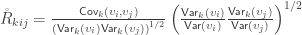
$\mathring{R}_{kij} = \frac{\mathsf{Cov}_k(\upsilon_i,\upsilon_j)}{\left(\mathsf{Var}_k(\upsilon_i)\mathsf{Var}_k(\upsilon_j)\right)^{1/2}} \left(\frac{\mathsf{Var}_k(\upsilon_i)}{\mathsf{Var}(\upsilon_i)}\frac{\mathsf{Var}_k(\upsilon_j)}{\mathsf{Var}(\upsilon_j)}\right)^{1/2}$

When $\mathbf{S}_k = 2\cdot\boldsymbol{\Phi}$ , the above reduces to $\mathring{R}_{kij} = \rho_k \sqrt{h^2_i h^2_j}$ , which is the signed version of $\text{\textsc{erv}}=\left|\rho_g\sqrt{h_i^2h_j^2}\right|$ when $k$ is the genetic component.

Positive-definiteness

$\mathbf{R}$ and $\mathbf{R}_k$ are covariance matrices and so, are positive-definite, whereas the correlation matrices $\mathbf{\mathring{R}}$ , $\mathbf{\mathring{R}}_k$ and $\mathbf{\breve{R}}_k$ are positive-semidefinite. A hybrid matrix that does not have to be positive-definite or semidefinite is:

$\mathbf{\check{R}}_k = \mathbf{I} \odot \mathbf{\mathring{R}}_k + \left(\mathbf{J}-\mathbf{I}\right) \odot \mathbf{\breve{R}}_k$

where $\mathbf{J}$ is a matrix of ones, $\mathbf{I}$ is the identity, both of size $T \times T$ , and $\odot$ is the Hadamard product. An example of such matrix of practical use is to show concisely the heritabilities for each trait in the diagonal and the genetic correlations in the off-diagonal.

Cauchy-Schwarz

Algorithmic advantages can be obtained from the positive-definiteness of $\mathbf{\mathring{R}}_k$ . The Cauchy–Schwarz theorem (Cauchy, 1821; Schwarz, 1888) states that:

$\mathring{R}_{kij} \leqslant \sqrt{\mathring{R}_{kii}\mathring{R}_{kjj}}$

Hence, the bounds for the off-diagonal elements can be known from the diagonal elements, which, by their turn, are estimated in a simpler, univariate model.

The Cauchy-Schwarz inequality imposes limits on the off-diagonal values of the matrix that contains the genetic covariances (or bivariate heritabilities).

Parameter estimation

Under the multivariate normal assumption, the parameters can be estimated maximising the following loglikelihood function:

$\mathcal{L}\left(\mathbf{R}_k,\boldsymbol{\beta}\Big|\mathbf{y},\mathbf{\tilde{X}}\right) = -\frac{1}{2} \left(N \ln 2\pi + \ln \left|\boldsymbol{\Omega}\right| + \left(\mathbf{y}-\mathbf{\tilde{X}}\boldsymbol{\beta}\right)'\boldsymbol{\Omega}\left(\mathbf{y}-\mathbf{\tilde{X}}\boldsymbol{\beta}\right)\right)$

where $N=S \cdot T$ is the number of observations on the stacked vector $\mathbf{y}$ . Unbiased estimates for $\boldsymbol{\beta}$ , although inefficient and inappropriate for hypothesis testing, can be obtained with ordinary least squares (OLS).

Parametric inference

Hypothesis testing can be performed with the likelihood ratio test (LRT), i.e., the test statistic is produced by subtracting from the loglikelihood of the model in which all the parameters are free to vary ( $\mathcal{L}_1$ ), the loglikelihood of a model in which the parameters being tested are constrained to zero, the null model ( $\mathcal{L}_0$ ). The statistic is given by $\lambda = 2\left(\mathcal{L}_1-\mathcal{L}_0\right)$ (Wilks, 1938), which here is asymptotically distributed as a 50:50 mixture of a $\chi^2_0$ and $\chi^2_{\text{df}}$ distributions, where df is the number of parameters being tested and free to vary in the unconstrained model (Self and Liang, 1987). From this distribution the p-values can be obtained.

References

Almasy L, Blangero J. Multipoint quantitative-trait linkage analysis in general pedigrees. Am J Hum Genet. 1998 May;62(5):1198–211.
Almasy L, Dyer TD, Blangero J. Bivariate quantitative trait linkage analysis: pleiotropy versus co-incident linkages. Genet Epidemiol. 1997 Jan;14(6):953–8.
Cauchy, A-L. Œuvres Completes D’Augustin Cauchy (published in 1882). Vol. XV. Gauthier-Villars et Fils, Paris, 1821.
Eisenhart C. The assumptions underlying the analysis of variance. Biometrics. 1947;3(1):1–21.
Falconer DS, Mackay TFC. Introduction to Quantitative Genetics. Addison Wesley Longman, Harlow, Essex, UK, 1996.
Glahn DC, Curran JE, Winkler AM, Carless MA, Kent JW, Charlesworth JC, et al. High dimensional endophenotype ranking in the search for major depression risk genes. Biol Psychiatry. 2012 Jan 1;71(1):6–14.
Schwarz HA. Über ein Flächen kleinsten Flächeninhalts betreffendes Problem der Variationsrechnung. Acta Societatis Scientiarum Fennicæ XV, 319–332, 1888.
Self SG, Liang KY. Asymptotic properties of maximum likelihood estimators and likelihood ratio tests under nonstandard conditions. J Am Stat Assoc. 1987;82(398):605–10.
Wilks SS. The Large-Sample Distribution of the Likelihood Ratio for Testing Composite Hypotheses. Ann Math Stat. 1938;9(1):60–2.

The photograph at the top (elephants) is by Anja Osenberg and was generously released into public domain.

Genetic resemblance between relatives

Posted on 13.June.2015 by A. M. Winkler

How similar?

The degree of relationship between two related individuals can be estimated by the probability that a gene in one subject is identical by descent to the corresponding gene (i.e., in the same locus) in the other. Two genes are said to be identical by descent (ibd) if both are copies of the same ancestral gene. Genes that are not ibd may still be identical through separate mutations, and be therefore identical by state (ibs), though these will not be considered in what follows.

The coefficients below were introduced by Jacquard in 1970, in a book originally published in French, and translated to English in 1974. A similar content appeared in an article by the same author in the journal Biometrics in 1972 (see the references at the end).

Coefficients of identity

Consider a particular autosomal gene $G$ . Each individual has two copies, one from paternal, another from maternal origin; these can be indicated as $G_i^P$ and $G_i^M$ for individual $i$ . There are 15 exactly distinct ways (states) in which the $G$ can be identical or not identical between two individuals, as shown in the figure below.

To each of these states $S_{1, \ldots , 15}$ , a respective probability $\delta_{1, \ldots , 15}$ can be assigned; these are called coefficients of identity by descent. These probabilities can be calculated at every generation following very elementary rules. For most problems, however, the distinction between paternal and maternal origin of a gene is irrelevant, and some of the above states are equivalent to others. If these are condensed, we can retain 9 distinct ways, shown in the figure below:

As before, to each of these states $\Sigma_{1, \ldots , 9}$ , a respective probability $\Delta_{1, \ldots , 9}$ can be assigned; these are called condensed coefficients of identity by descent, and relate to the former as:

$\Delta_1 = \delta_1$
$\Delta_2 = \delta_6$
$\Delta_3 = \delta_2 + \delta_3$
$\Delta_4 = \delta_7$
$\Delta_5 = \delta_4 + \delta_5$
$\Delta_6 = \delta_8$
$\Delta_7 = \delta_9 + \delta_{12}$
$\Delta_8 = \delta_{10} + \delta_{11} + \delta_{13} + \delta_{14}$
$\Delta_9 = \delta_{15}$

A similar method was proposed by Cotterman (1940), in his highly influential but only much later published doctoral thesis. The $\Delta_9$ , $\Delta_8$ and $\Delta_7$ correspond to his coefficients $k_0$ , $k_1$ and $k_2$ .

Coefficient of kinship

The above refer to probabilities of finding particular genes as identical among subjects. However, a different coefficient can be defined for random genes: the probability that a random gene from subject $i$ is identical with a gene at the same locus from subject $j$ is the coefficient of kinship, and can be represented as $\phi_{ij}$ :

$\phi_{ij} = \Delta_1 + \frac{1}{2}(\Delta_3 + \Delta_5 + \Delta_7) + \frac{1}{4}\Delta_8$

If $i$ and $j$ are in fact the same individual, then $\phi_{ii}$ is the kinship of a subject with himself. Two genes taken from the same individual can either be the same gene (probability $\frac{1}{2}$ of being the same) or be the genes inherited from father and mother, in which case the probability is given by the coefficient of kinship between the parents. In other words, $\phi_{ii} = \frac{1}{2} + \frac{1}{2}\phi_{\text{FM}}$ . If both parents are unrelated, $\phi_{\text{FM}}=0$ , such that the kinship of a subject with himself is $\phi_{ii} = \frac{1}{2}$ .

The value of $\phi_{ij}$ can be determined from the number of generations up to a common ancestor $k$ . A random gene from individual $i$ can be identical to a random gene from individual $j$ in the same locus if both comes from the common ancestor $k$ , an event that can happen if either (1) both are copies of the gene in $k$ , or (2) if they are copies of different genes in $k$ , but $k$ is inbred; this has probability $\frac{1}{2}f_k$ (see below about the coefficient of inbreeding, $f$ ). Thus, if there are $m$ generations between $i$ and $k$ , and $n$ generations between $j$ and $k$ , the coefficient of kinship can be computed as $\phi_{ij} = \left(\frac{1}{2}\right)^{m+n+1}(1+f_k)$ . If $i$ and $j$ can have more than one common ancestor, then there are more than one line of descent possible, and the kinship is determined by integrating over all such possible $K$ common ancestors:

$\phi_{ij} = \sum_{k=1}^K \left(\frac{1}{2}\right)^{m_k+n_k+1}(1+f_k)$

For a set of subjects, the pairwise coefficients of kinship $\phi_{ij}$ can be arranged in a square matrix $\boldsymbol{\Phi}$ , and used to model the covariance between subjects as $2\cdot\boldsymbol{\Phi}$ (see here).

Coefficient of inbreeding

The coefficient of inbreeding $f$ of a given subject $i$ is the coefficient of kinship between their parents. While the above coefficients provide information about pairs of individuals, the coefficient of inbreeding gives information about a particular subject. Yet, $f_i$ can be computed from the coefficients of identity:

$f_{i} = \Delta_1 + \Delta_2 + \Delta_3 + \Delta_4$
$f_{j} = \Delta_1 + \Delta_2 + \Delta_5 + \Delta_6$

Note that all these coefficients are based on probabilities, but it is now possible to identify the actual presence of a particular gene using marker data. Also note that while the illustrations above suggest application to livestock, the same applies to studies of human populations.

Some particular cases

The computation of the above coefficients can be done using algorithms, and are done automatically by software that allow analyses of pedigree data, such as solar. Some common particular cases are shown below:

Relationship	$\Delta_1$	$\Delta_2$	$\Delta_3$	$\Delta_4$	$\Delta_5$	$\Delta_6$	$\Delta_7$	$\Delta_8$	$\Delta_9$	$\phi_{ij}$
Self	$0$	$0$	$0$	$0$	$0$	$0$	$1$	$0$	$0$	$\frac{1}{2}$
Parent-offspring	$0$	$0$	$0$	$0$	$0$	$0$	$0$	$1$	$0$	$\frac{1}{4}$
Half sibs	$0$	$0$	$0$	$0$	$0$	$0$	$0$	$\frac{1}{2}$	$\frac{1}{2}$	$\frac{1}{8}$
Full sibs/dizygotic twins	$0$	$0$	$0$	$0$	$0$	$0$	$\frac{1}{4}$	$\frac{1}{2}$	$\frac{1}{4}$	$\frac{1}{4}$
Monozygotic twins	$0$	$0$	$0$	$0$	$0$	$0$	$1$	$0$	$0$	$\frac{1}{2}$
First cousins	$0$	$0$	$0$	$0$	$0$	$0$	$0$	$\frac{1}{4}$	$\frac{3}{4}$	$\frac{1}{16}$
Double first cousins	$0$	$0$	$0$	$0$	$0$	$0$	$\frac{1}{16}$	$\frac{6}{16}$	$\frac{9}{16}$	$\frac{1}{8}$
Second cousins	$0$	$0$	$0$	$0$	$0$	$0$	$0$	$\frac{1}{16}$	$\frac{15}{16}$	$\frac{1}{64}$
Uncle-nephew	$0$	$0$	$0$	$0$	$0$	$0$	$0$	$\frac{1}{2}$	$\frac{1}{2}$	$\frac{1}{8}$
Offspring of sib-matings	$\frac{1}{16}$	$\frac{1}{32}$	$\frac{1}{8}$	$\frac{1}{32}$	$\frac{1}{8}$	$\frac{1}{32}$	$\frac{7}{32}$	$\frac{5}{16}$	$\frac{1}{16}$	$\frac{3}{8}$

References

Cotterman C. A calculus for statistico-genetics. 1940. PhD Thesis. Ohio State University.
Jacquard, A. Structures génétiques des populations. Masson, Paris, France, 1970, later translated and republished as Jacquard, A. The genetic structure of populations. Springer, Heidelberg, 1974.
Jacquard A. Genetic information given by a relative. Biometrics. 1972;28(4):1101-1114.

The photograph at the top (sheep) is in public domain.