September | 2015 | Brainder.

In a previous post, all commonly used univariate and multivariate test statistics used with the general linear model (GLM) were presented. Here an alternative formulation for one of these statistics, the Pillai’s trace (Pillai, 1955, references at the end), commonly used in MANOVA and MANCOVA tests, is presented.

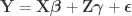
We begin with a multivariate general linear model expressed as:

$\mathbf{Y} = \mathbf{M} \boldsymbol{\psi} + \boldsymbol{\epsilon}$

where $\mathbf{Y}$ is the $N \times K$ full rank matrix of observed data, with $N$ observations of $K$ distinct (possibly non-independent) variables, $\mathbf{M}$ is the full-rank $N \times R$ design matrix that includes explanatory variables (i.e., effects of interest and possibly nuisance effects), $\boldsymbol{\psi}$ is the $R \times K$ vector of $R$ regression coefficients, and $\boldsymbol{\epsilon}$ is the $N \times K$ vector of random errors. Estimates for the regression coefficients can be computed as $\boldsymbol{\hat{\psi}} = \mathbf{M}^{+}\mathbf{Y}$ , where the superscript ( $^{+}$ ) denotes a pseudo-inverse.

The null hypothesis, and a simplification

One is generally interested in testing the null hypothesis that a contrast of regression coefficients is equal to zero, i.e., $\mathcal{H}_{0} : \mathbf{C}'\boldsymbol{\psi}\mathbf{D} = \boldsymbol{0}$ , where $\mathbf{C}$ is a $R \times S$ full-rank matrix of $S$ contrasts of coefficients on the regressors encoded in $\mathbf{X}$ , $1 \leqslant S \leqslant R$ and $\mathbf{D}$ is a $K \times Q$ full-rank matrix of $Q$ contrasts of coefficients on the dependent, response variables in $\mathbf{Y}$ , $1 \leqslant Q \leqslant K$ ; if $K=1$ or $Q=1$ , the model is univariate. Once the hypothesis has been established, $\mathbf{Y}$ can be equivalently redefined as $\mathbf{Y}\mathbf{D}$ , such that the contrast $\mathbf{D}$ can be omitted for simplicity, and the null hypothesis stated as $\mathcal{H}_{0} : \mathbf{C}'\boldsymbol{\psi} = \boldsymbol{0}$ .

Model partitioning

It is useful to consider a transformation of the model into a partitioned one:

$\mathbf{Y} = \mathbf{X}\boldsymbol{\beta} + \mathbf{Z}\boldsymbol{\gamma} + \boldsymbol{\epsilon}$

where $\mathbf{X}$ is the matrix with regressors of interest, $\mathbf{Z}$ is the matrix with nuisance regressors, and $\boldsymbol{\beta}$ and $\boldsymbol{\gamma}$ are respectively the vectors of regression coefficients. From this model we can also define the projection (hat) matrices $\mathbf{H}_{\mathbf{X}}=\mathbf{X}\mathbf{X}^{+}$ and $\mathbf{H}_{\mathbf{Z}}=\mathbf{Z}\mathbf{Z}^{+}$ due to tue regressors of interest and nuisance, respectively, and the residual-forming matrices $\mathbf{R}_{\mathbf{X}}=\mathbf{I}-\mathbf{H}_{\mathbf{X}}$ and $\mathbf{R}_{\mathbf{Z}}=\mathbf{I}-\mathbf{H}_{\mathbf{Z}}$ .

Such partitioning is not unique, and schemes can be as simple as separating apart the columns of $\mathbf{M}$ as $\left[ \mathbf{X} \; \mathbf{Z} \right]$ , with $\boldsymbol{\psi} = \left[ \boldsymbol{\beta}' \; \boldsymbol{\gamma}' \right]'$ . More involved strategies can, however, be devised to obtain some practical benefits. One such partitioning is to define $\mathbf{X} = \mathbf{M} \mathbf{Q} \mathbf{C} \left(\mathbf{C}'\mathbf{Q}\mathbf{C}\right)^{-1}$ and
$\mathbf{Z} = \mathbf{M} \mathbf{Q} \mathbf{C}_v \left(\mathbf{C}_v'\mathbf{Q}\mathbf{C}_v\right)^{-1}$ , where $\mathbf{Q}=(\mathbf{M}'\mathbf{M})^{-1}$ , $\mathbf{C}_v=\mathbf{C}_u-\mathbf{C}(\mathbf{C}'\mathbf{Q}\mathbf{C})^{-1}\mathbf{C}'\mathbf{Q}\mathbf{C}_u$ , and $\mathbf{C}_u$ has $r-\mathsf{rank}\left(\mathbf{C}\right)$ columns that span the null space of $\mathbf{C}$ , such that $[\mathbf{C} \; \mathbf{C}_u]$ is a $r \times r$ invertible, full-rank matrix (Smith et al, 2007). This partitioning has a number of features: $\boldsymbol{\hat{\beta}} = \mathbf{C}'\boldsymbol{\hat{\psi}}$ , $\widehat{\mathsf{Cov}}(\boldsymbol{\hat{\beta}}) = \mathbf{C}'\widehat{\mathsf{Cov}}(\boldsymbol{\hat{\psi}})\mathbf{C}$ , i.e., estimates and variances of $\boldsymbol{\beta}$ for inference on the partitioned model correspond exactly to the same inference on the original model, $\mathbf{X}$ is orthogonal to $\mathbf{Z}$ , and $\mathsf{span}(\mathbf{X}) \cup \mathsf{span}(\mathbf{Z}) = \mathsf{span}(\mathbf{M})$ , i.e., the partitioned model spans the same space as the original.

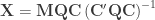
Another partitioning scheme, derived by Ridgway (2009), defines $\mathbf{X}=\mathbf{M}(\mathbf{C}^+)'$ and $\mathbf{Z}=\mathbf{M}-\mathbf{M}\mathbf{C}\mathbf{C}^{+}$ . As with the previous strategy, the parameters of interest in the partitioned model are equal to the contrast of the original parameters. A full column rank nuisance partition can be obtained from the singular value decomposition (SVD) of $\mathbf{Z}$ , which will also provide orthonormal columns for the nuisance partition. Orthogonality between regressors of interest and nuisance can be obtained by redefining the regressors of interest as $\mathbf{R}_{\mathbf{Z}}\mathbf{X}$ .

The usual multivariate statistics

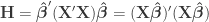
For the multivariate statistics, define generically:

$\mathbf{H}=(\mathbf{C}'\boldsymbol{\hat{\psi}}\mathbf{D})' \left(\mathbf{C}'(\mathbf{M}'\mathbf{M})^{-1}\mathbf{C} \right)^{-1} (\mathbf{C}'\boldsymbol{\hat{\psi}}\mathbf{D})$

as the sums of products explained by the model (hypothesis) and:

$\mathbf{E} = (\boldsymbol{\hat{\epsilon}}\mathbf{D})'(\boldsymbol{\hat{\epsilon}}\mathbf{D})$

as the sums of the products of the residuals, i.e., that remain unexplained. With the simplification to the original model that redefined $\mathbf{Y}$ as $\mathbf{Y}\mathbf{D}$ , the $\mathbf{D}$ can be dropped, so that we have $\mathbf{H}=(\mathbf{C}'\boldsymbol{\hat{\psi}})' \left(\mathbf{C}'(\mathbf{M}'\mathbf{M})^{-1}\mathbf{C} \right)^{-1} (\mathbf{C}'\boldsymbol{\hat{\psi}})$ and $\mathbf{E} = \boldsymbol{\hat{\epsilon}}'\boldsymbol{\hat{\epsilon}}$ . The various well-known multivariate statistics (see this earlier blog entry) can be written as a function of $\mathbf{H}$ and $\mathbf{E}$ . Pillai’s trace is:

$T=\mathsf{trace}\left(\mathbf{H}(\mathbf{H}+\mathbf{E})^{-1}\right)$

More simplifications

With the partitioning, other simplifications are possible:

$\mathbf{H}=\boldsymbol{\hat{\beta}}' (\mathbf{X}'\mathbf{X})\boldsymbol{\hat{\beta}} = ( \mathbf{X}\boldsymbol{\hat{\beta}})'(\mathbf{X}\boldsymbol{\hat{\beta}})$

Recalling that $\mathbf{X}'\mathbf{Z}=\mathbf{0}$ , and defining $\tilde{\mathbf{Y}}=\mathbf{R}_{\mathbf{Z}}\mathbf{Y}$ , we have:

$\mathbf{H} = (\mathbf{H}_{\mathbf{X}}\tilde{\mathbf{Y}})'(\mathbf{H}_{\mathbf{X}}\tilde{\mathbf{Y}}) = \tilde{\mathbf{Y}}'\mathbf{H}_{\mathbf{X}}\tilde{\mathbf{Y}}$

The unexplained sums of products can be written in a similar manner:

$\mathbf{E} = (\mathbf{R}_{\mathbf{X}}\tilde{\mathbf{Y}})'(\mathbf{R}_{\mathbf{X}}\tilde{\mathbf{Y}}) = \tilde{\mathbf{Y}}'\mathbf{R}_{\mathbf{X}}\tilde{\mathbf{Y}}$

The term $\mathbf{H}+\mathbf{E}$ in the Pillai’s trace can therefore be rewritten as:

$\mathbf{H}+\mathbf{E}= \tilde{\mathbf{Y}}'(\mathbf{H}_{\mathbf{X}} + \mathbf{R}_{\mathbf{X}})\tilde{\mathbf{Y}} = \tilde{\mathbf{Y}}'\tilde{\mathbf{Y}}$

Using the property that the trace of a product is invariant to a circular permutation of the factors, Pillai’s statistic can then be written as:

$\begin{array}{ccl} T&=&\mathsf{trace}\left(\tilde{\mathbf{Y}}'\mathbf{H}_{\mathbf{X}}\tilde{\mathbf{Y}}\left(\tilde{\mathbf{Y}}'\tilde{\mathbf{Y}}\right)^{+}\right)\\ {}&=&\mathsf{trace}\left(\mathbf{H}_{\mathbf{X}}\tilde{\mathbf{Y}}\left(\tilde{\mathbf{Y}}'\tilde{\mathbf{Y}}\right)^{+}\tilde{\mathbf{Y}}'\right)\\ {}&=&\mathsf{trace}\left(\mathbf{H}_{\mathbf{X}}\tilde{\mathbf{Y}}\tilde{\mathbf{Y}}^{+}\right)\\ \end{array}$

The final, alternative form

Using sigular value decomposition we have $\tilde{\mathbf{Y}} = \mathbf{U}\mathbf{S}\mathbf{V}'$ and $\tilde{\mathbf{Y}}^{+} = \mathbf{V}\mathbf{S}^{+}\mathbf{U}'$ , where $\mathbf{U}$ contains only the columns that correspond to non-zero eigenvalues. Thus, the above can be rewritten as:

$\begin{array}{ccl} T&=&\mathsf{trace}\left(\mathbf{H}_{\mathbf{X}} \mathbf{U}\mathbf{S}\mathbf{V}' \mathbf{V}\mathbf{S}^{+}\mathbf{U}' \right)\\ {}&=&\mathsf{trace}\left(\mathbf{H}_{\mathbf{X}} \mathbf{U}\mathbf{U}' \right)\\ \end{array}$

The SVD transformation is useful for languages or libraries that offer a fast implementation. Otherwise, using a pseudoinverse yields the same result, perhaps only slightly slower. In this case, $T=\mathsf{trace}\left(\mathbf{H}_{\mathbf{X}}\tilde{\mathbf{Y}}\tilde{\mathbf{Y}}^{+}\right)$ .

Importance

If we define $\mathbf{A}\equiv\mathbf{H}_{\mathbf{X}}$ and $\mathbf{W}\equiv\mathbf{U}\mathbf{U}'$ (or $\mathbf{W}\equiv\tilde{\mathbf{Y}}\tilde{\mathbf{Y}}^{+}$ ), then $T=\mathsf{trace}\left(\mathbf{A}\mathbf{W}\right)$ . The first three moments of the permutation distribution of statistics that can be written in this form can be computed analytically once $\mathbf{A}$ and $\mathbf{W}$ are known. With the first three moments, a gamma distribution (Pearson type III) can be fit, thus allowing p-values to be computed without resorting to the usual beta approximation to Pillai’s trace, nor using permutations, yet with results that are not based on the assumption of normality (Mardia, 1971; Kazi-Aoual, 1995; Minas and Montana, 2014).

Availability

This simplification is available in PALM, for use with imaging and non-imaging data, using Pillai’s trace itself, or a modification that allows inference on univariate statistics. As of today, this option is not yet documented, but should become openly available soon.

References

Kazi-Aoual F, Hitier S, Sabatier R, Lebreton J-D. Refined approximations to permutation tests for multivariate inference. Comput Stat Data Anal. 1995;20(94):643–56.
Mardia KV. The Effect of Nonnormality on some multivariate tests and robustness to nonnormality in the linear model. Biometrika. 1971;58(1):105–21.
Minas C, Montana G. Distance-based analysis of variance: Approximate inference. Stat Anal Data Min. 2014;7(6):450–70.
Pillai KCS. Some New test criteria in multivariate analysis. Ann Math Stat. 1955;26(1):117–21.
Ridgway GR. Statistical analysis for longitudinal MR imaging of dementia. PhD Thesis. University College London, 2009.
Smith SM, Jenkinson M, Beckmann CF, Miller K, Woolrich M. Meaningful design and contrast estimability in FMRI. Neuroimage. 2007;34(1):127–36.
Winkler AM, Ridgway GR, Webster MA, Smith SM, Nichols TE. Permutation inference for the general linear model. Neuroimage. 2014;92:381–97.

Update: 20.Jan.2016: A slight simplification was applied to the formulas above so as to make them more elegant and remove some redundancy. The result is the same.