Have you ever had an analysis in which there was a large set of contrasts, all of interest, and you were worried about multiple testing? An eventual effect would be missed by a simple Bonferroni correction, but you did not know what else to do? Or did you have a set of different studies and you wished to obtain a style of meta-analytic result, indicating whether there would be evidence across all of them, without requiring the studies to be all consistently significant?
The Non-Parametric Combination (NPC) solves these issues. It is a way of performing joint inference on multiple data collected on the same experimental units (e.g., same subjects), all with minimal assumptions. The method was proposed originally by Pesarin (1990, 1992) [see references below], independently by Blair and Karninski (1993), and described extensively by Pesarin and Salmaso (2010). In this blog entry, the NPC is presented in brief, with emphasis on the modifications we introduce to render it feasible for brain imaging. The complete details are in our paper that has just been published in the journal Human Brain Mapping.
NPC in a nutshell
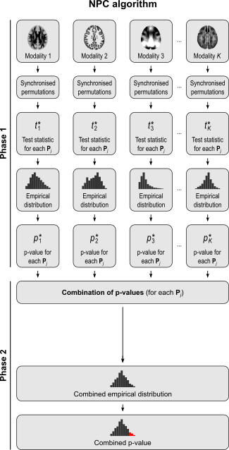
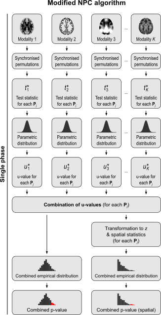
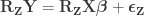
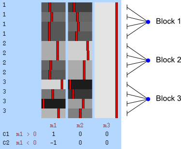
The NPC consists of, in a first phase, testing each hypothesis separately using permutations that are performed synchronously across datasets; these tests are termed partial tests. The resulting statistics for each and every permutation are recorded, allowing an estimate of the complete empirical null distribution to be constructed for each one. In a second phase, the empirical p-values for each statistic are combined, for each permutation, into a joint statistic. As such a combined joint statistic is produced from the previous permutations, an estimate of its empirical distribution function is immediately known, and so is the p-value of the joint test. A flowchart of the original algorithm is shown below; click to see it side-by-side with the modified one (described below).
A host of combining functions
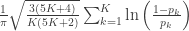
The null hypothesis of the NPC is that null hypotheses for all partial tests are true, and the alternative hypothesis that any is false, which is the same null of a union-intersection test (UIT; Roy, 1953). The rejection region depends on how the combined statistic is produced. Various combining functions, which produce such combined statistics, can be considered, and some of the most well known are listed in the table below:
| Method |
Statistic |
p-value |
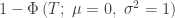
| Tippett |
 |
 |
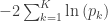
| Fisher |
 |
 |
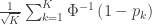
| Stouffer |
 |
 |
| Mudholkar–George |
 |
 |
In the table,  is the number of partial tests, and the remaining of the variables follow the usual notation (see the Table 1 in the paper for the complete description). Many of these combining functions were proposed over the years for applications such as meta-analyses, and many of them assume independence between the tests being combined, and will give incorrect p-values if such assumption is not met. In the NPC, lack of dependence is not a problem, even if these same functions are used: the synchronised permutations ensure that any dependence, if existing, is taken into account, and this is done so implicitly, with no need for explicit modelling.
The different combining functions lead to different rejection regions for the null hypothesis. For the four combining functions in the table above, the respective rejection regions are in the figure below.
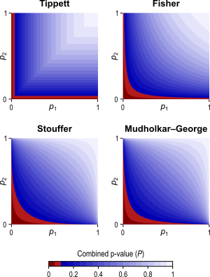
The combining functions can be modified to allow combination of tests so as to favour hypotheses with concordant directions, or be modified for bi-directional tests. Click on the figure above for examples of these cases (again, see the paper for the complete details).
Two problems, one solution
The multiple testing problem is well known in brain imaging: as an image comprises thousands of voxels/vertices/faces, correction is necessary. Bonferroni is in general too conservative, and various other approaches have been proposed, such as the random field theory. Permutation tests provide control over the familywise error rate (FWER) for the multiple tests across space, requiring only the assumption of exchangeability. This is all well known; see Nichols and Hayasaka (2003) and Winkler et al. (2014) for details.
However, another type of multiple testing is also common: analyses that test multiple hypotheses using the same model, multiple pairwise group comparisons, multiple and distinct models, studies using multiple modalities, that mix imaging and non-imaging data, that consider multiple processing pipelines, and even multiple multivariate analyses. All these common cases also need multiple testing correction. We call this multiple testing problem MTP-II, to discern it from the well known multiple testing problem across space, described above, which we term MTP-I.
One of the many combining functions possible with NPC, the one proposed by Tippett (1931), has a further property that makes it remarkably interesting. The Tippett function uses the smallest p-value across partial tests as its test statistic. Alternatively, if all statistics are comparable, it can be formulated in terms of the maximum statistic. It turns out that the distribution of the maximum statistic across a set of tests is also the distribution that can be used in a closed testing procedure (Marcus et al., 1976) to correct for the familywise error rate (FWER) using resampling methods, such as permutation. In the context of joint inference, FWER-correction can also be seen as an UIT. Thus, NPC offers a link between combination of multiple tests, and correction for multiple tests, in both cases regardless of any dependence between such tests.
This means that the MTP-II, for which correction in the parametric realm is either non-existing or fiendishly difficult, can be accommodated easily. It requires no explicit modelling of the dependence between the tests, and the resulting error rates are controlled exactly at the test level, adding rigour to what otherwise could lead to an excess of false positives without correction, or be overly conservative if a naïve correction such as Bonferroni were attempted.
Modifying for imaging applications
As originally proposed, in practice NPC cannot be used in brain imaging. As the statistics for all partial tests for all permutations need to be recorded, an enormous amount of space for data storage is necessary. Even if storage space were not a problem, the discreteness of the p-values for the partial tests is problematic when correcting for multiple testing, because with thousands of tests in an image, ties are likely to occur, further causing ties among the combined statistics. If too many tests across an image share the same most extreme statistic, correction for the MTP-I, while still valid, becomes less powerful (Westfall and Young, 1993; Pantazis et al., 2005). The most obvious workaround — run an ever larger number of permutations to break the ties — may not be possible for small sample sizes, or when possible, requires correspondingly larger data storage.
The solution is loosely based on the direct combination of the test statistics, by converting the test statistics of the partial tests to values that behave as p-values, using the asymptotic distribution of the statistics for the partial tests. We call these as “u-values”, in order to emphasise that they are not meant to be read or interpreted as p-values, but rather as transitional values that allow combinations that otherwise would not be possible.
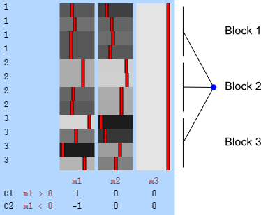
For spatial statistics, the asymptotic distribution of the combined statistic is used, this time to produce a z-score, which can be subjected to the computation of cluster extent, cluster mass, and/or threshold-free cluster enhancement (TFCE; Smith and Nichols, 2009). A flow chart of the modified algorithm is shown below. Click to see it side-by-side with the original.
More power, fewer assumptions
One of the most remarkable features of NPC is that the synchronised permutations implicitly account for the dependence structure among the partial tests. This means that even combining methods originally derived under the assumption of independence can be used when such independence is untenable. As the p-values are assessed via permutations, distributional restrictions are likewise not necessary, liberating NPC from most assumptions that thwart parametric methods in general. This renders NPC a good alternative to classical multivariate tests, such as MANOVA, MANCOVA, and Hotelling’s T2 tests: each of the response variables can be seen as an univariate partial test in the context of the combination, but without the assumptions that are embodied in these old multivariate tests.
As if all the above were not already sufficient, NPC is also more powerful than such classical multivariate tests. This refers to its finite sample consistency property, that is, even with fixed sample size, as the number of modalities being combined increases, the power of the test also increases. The power of classical multivariate tests, however, increases up to a certain point, then begins to decrease, eventually reaching zero when the number of combining variables match the sample size.
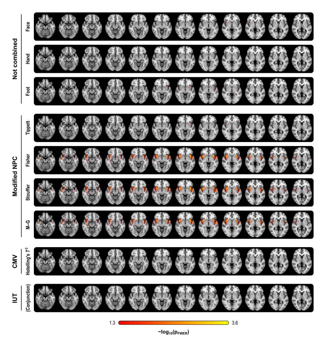
The figure below summarises the analysis of a subset of the subjects of a published FMRI study (Brooks et al, 2005) in which painful stimulation was applied to the face, hand, and foot of 12 subjects. Using permutation tests separately, no results could be identified for any of the three types of stimulation. A simple multivariate test, the Hotelling’s T2 test, even assessed using permutations, did not reveal any effect of stimulation either. The NPC results, however, suggest involvement of large portions of the anterior insula and secondary somatosensory cortex. The Fisher, Stouffer and Mudholkar–George combining functions were particularly successful in recovering a small area of activity in the midbrain and periaqueductal gray area, which would be expected from previous studies on pain, but that could not be located from the original, non-combined data.
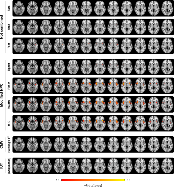
Detailed assessment of power, using variable number of modalities, and of modalities containing signal, is shown in the paper.
Combinations or conjunctions?
Combination, as done via NPC, is different than conjunctions (Nichols et al., 2005) in the following: in the combination, one seeks for aggregate significance across partial tests, without the need that any individual study is necessarily significant. In the conjunction, it is necessary that all of them, with no exception, is significant. As indicated above, the NPC forms an union-intersection test (UIT; Roy, 1953), whereas the conjunctions form an intersection-union test (IUT; Berger, 1982). The former can be said to be significant if any (or an aggregate) of the partial tests is significant, whereas the latter is significant if all the partial tests are.
Availability
The NPC, with the modifications for brain imaging, is available in the tool PALM — Permutation Analysis of Linear Models. It runs in either Matlab or Octave, and is free (GPL).
References
- Berger RL. Multiparameter hypothesis testing and acceptance sampling. Technometrics. 1982;24(4):295-300.
- Blair RC, Karniski W. An alternative method for significance testing of waveform difference potentials. Psychophysiology. 1993;30(5):518-24.
- Brooks JCW, Zambreanu L, Godinez A, Craig ADB, Tracey I. Somatotopic organisation of the human insula to painful heat studied with high resolution functional imaging. Neuroimage. 2005;27(1):201-9.
- Nichols T, Brett M, Andersson J, Wager T, Poline J-B. Valid conjunction inference with the minimum statistic. Neuroimage. 2005 Apr 15;25(3):653-60.
- Nichols T, Hayasaka S. Controlling the familywise error rate in functional neuroimaging: a comparative review. Stat Methods Med Res. 2003 Oct;12(5):419-46.
- Pantazis D, Nichols TE, Baillet S, Leahy RM. A comparison of random field theory and permutation methods for the statistical analysis of MEG data. Neuroimage. 2005;25(2):383-94.
- Pesarin F. On a nonparametric combination method for dependent permutation tests with applications. Psychother Psychosom. 1990;54:172-9.
- Pesarin F. A resampling procedure for nonparametric combination of several dependent tests. J Ital Stat Soc. 1992;1(1):87-101.
- Pesarin F, Salmaso L. Permutation Tests for Complex Data: Theory, Applications and Software. John Wiley and Sons, West Sussex, England, UK, 2010.
- Roy SN. On a Heuristic Method of Test Construction and its use in Multivariate Analysis. Ann Math Stat. 1953 Jun;24(2):220-38.
- Smith SM, Nichols TE. Threshold-free cluster enhancement: addressing problems of smoothing, threshold dependence and localisation in cluster inference. Neuroimage. 2009;44(1):83-98.
- Tippett LHC. The methods of statistics. Williams and Northgate, London, 1931.
- Westfall PH, Young SS. Resampling-Based Multiple Testing: Examples and Methods for p-Value Adjustment. John Wiley and Sons, New York, 1993.
- Winkler AM, Ridgway GR, Webster MA, Smith SM, Nichols TE. Permutation inference for the general linear model. Neuroimage. 2014;92:381-97 (Open Access).
- Winkler AM, Webster MA, Brooks JC, Tracey I, Smith SM, Nichols TE. Non-parametric combination and related permutation tests for neuroimaging. Hum Brain Mapp. 2016 Feb 5 (in press, Open Access). The Supporting Information can be browsed directly here. This paper supersedes our earlier poster presented in the 2013 OHBM conference.
Contributed to this post: Tom Nichols.


. Use the estimated parameters
to compute the statistic of interest, and call this statistic
.
, obtaining estimated parameters
and estimated residuals
.
. This is done by pre-multiplying the residuals from the reduced model produced in the previous step,
, then adding back the estimated nuisance effects, i.e.
.
to compute the statistic of interest. Call this statistic
.
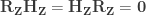
under the null hypothesis of no association between


, implying that the permutations can actually be performed just by permuting the rows of the residual-forming matrix
.


 be a sequence of independent and identically distributed variables with cumulative distribution function (cdf)
  and let
  denote the maximum.
 directly is problematic because as
  ,
,  . Redefining the problem as a function of
  renders treatment simpler. The theorem can be stated then as: If there exist sequences of constants
  and
and  such that, as
 belongs to one of three “domains of attraction”:
 , for
, for  indicating that the distribution of
  indicating that the distribution of
  indicating that the distribution of
  ,
,  and, for families II and III,
  . To which of the three a particular
  . Thus, we can infer about the asymptotic properties of the maximum while having only a limited knowledge of the properties of
  , whereas Fisher and Tippett used
 , with parameters
  (location),
  (scale), and
  (shape). This is the generalised extreme value (GEV) family of distributions. If
  , it converges to Gumbel (type I), whereas if
  it corresponds to Fréchet (type II), and if
  it corresponds to Weibull (type III). Inference on
  allows choice of a particular family for a given problem.
 , the limiting distribution of a random variable
  , conditional on
  , is:
, is:
 and
and  . The two parameters are the
  (scale). The shape corresponds to the same parameter
  .
. as
as ![\left[0, \tilde{\sigma}\right]](https://s0.wp.com/latex.php?latex=%5Cleft%5B0%2C+%5Ctilde%7B%5Csigma%7D%5Cright%5D&bg=ffffff&fg=333333&s=0&c=20201002) when
when  , and a Pareto distribution when
  .
. , which represent distributions approximately exponential, parametters for the GPD can be estimated using at least three methods: maximum likelihood, moments, and probability-weighted moments. These are described in Hosking and Wallis (1987). For
  and
and  be respectively the sample mean and variance. The moment estimators of
  and
and  .
.


 distinct possible orderings of these cups, and by telling the subject in advance that there are four cups of each type, this guarantees that the answer will include four of each.
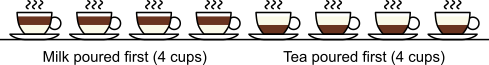


 . This is not the final result, though: what matters to disprove the hypothesis that she is not able to discriminate is how likely it would be for her to find a result at least as extreme as the one observed. In this case, there is one case that is more extreme, which would be the one in which she would have made correct guesses for all the 8 cups, in which case the values in the contingency table above would have been
  ,
,  ,
,  , and
, and  , with a probability computed with the same formula as
  . Adding these two probabilities together yield
  .
.

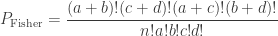
 . Computing from the above (details omitted), yield the same value as using Fisher’s presentation, that is, the p-value is (exactly) 0.24286.
 method
 is the observed value for the element in the position
  in the table,
  and
and  are respectively the number of rows and columns, and
  is the expected value for these elements if the null hypothesis is true. The values
  and column
  . A simpler, equivalent formula is given by:
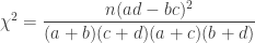
 .
. , which corresponds to a p-value of 0.07865. However, it is well known that this method is inaccurate if cells in the table have too small quantities, usually below 5 or 6.
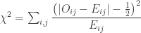
 , and a p-value of 0.23975, which is very similar to the one given by the Fisher method. Note again that this approach, like the
  be a column vector containing binary indicators for whether milk was truly poured first. Let
  be a column vector containing binary indicators for whether the lady answered that milk was poured first. The
  , where
  is a regression coefficient, and
  possible unique rearrangements. Out of these, in 17, there are 6 or more (out of 8) correct answers matching the values in
 contains the regressors,
  the regression coefficients, which are to be estimated, and
  , where
  is a contrast. If
  , the Student’s t statistic can be calculated as:
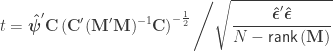
 and
and  indicate that these are quantities estimated from the sample. If
  , the F statistic can be obtained as:
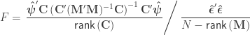
 . For either of these statistics, we can assess their significance by repeating the same fit after permuting
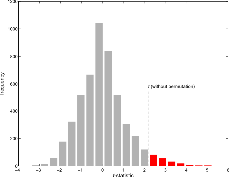
 is a diagonal matrix that has elements:
 are the
  diagonal elements of the residual forming matrix, and
  is the variance group to which the
  , is given by
 . The matrix
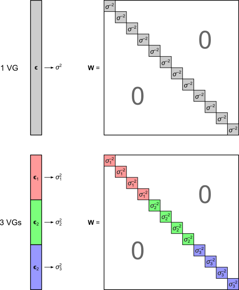
 , the t-equivalent to the G-statistic is
  , which is the well known Aspin-Welch
  -statistic for the Behrens-Fisher problem. The relationship between

 and
and  .
.

 is the estimated p-value,
  is the number of permutations,
  is the statistic for the unpermuted model,
  is the statistic for the
  is an indicator function that evaluates as 1 if the condition between parenthesis is true, or 0 otherwise. This formulation produces unbiased results: since
  , the true p-value, then
  .
. , is small, or if the number of permutations is not sufficiently large, even after all the
  may reach or surpass the value of
  :
:
 ,
,  , and so,
  .
. , in a way that no p-value smaller than
