randomise | Brainder.

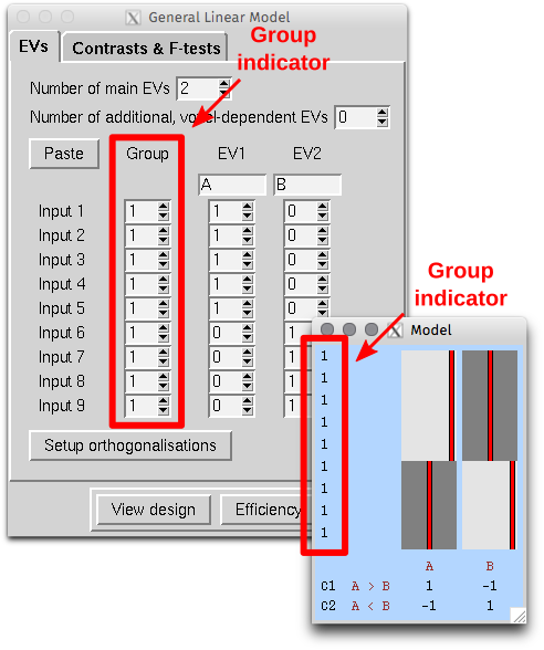
In FSL, when we create a design using the graphical interface in FEAT, or with the command Glm, we are given the opportunity to define, at the higher-level, the “Group” to which each observation belongs. When the design is saved, the information from this setting is stored in a text file named something as “design.grp”. This file, and thus the group setting, takes different roles depending whether the analysis is used in FEAT itself, in PALM, or in randomise.

What can be confusing sometimes is that, in all three cases, the “Group” indicator does not refer to experimental or observational group of any sort. Instead, it refers to variance groups (VG) in FEAT, to exchangeability blocks (EB) in randomise, and to either VG or EB in PALM, depending on whether the file is supplied with the options -vg or -eb.

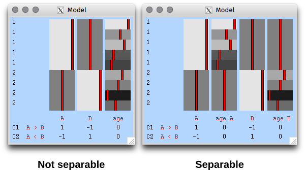
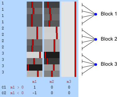
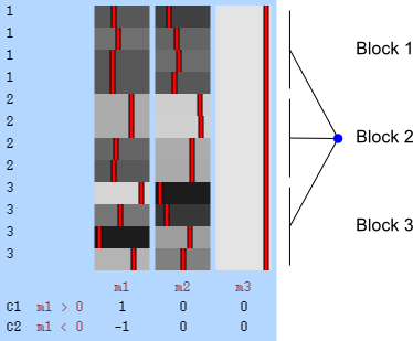
In FEAT, unless there is reason to suspect (or assume) that the variances for different observations are not equal, all subjects should belong to group “1”. If variance groups are defined, then these are taken into account when the variances are estimated. This is only possible if the design matrix is “separable”, that is, it must be such that, if the observations are sorted by group, the design can be constructed by direct sum (i.e., block-diagonal concatenation) of the design matrices for each group separately. A design is not separable if any explanatory variable (EV) present in the model crosses the group borders (see figure below). Contrasts, however, can encompass variables that are defined across multiple VGs.

The variance groups not necessarily must match the experimental observational groups that may exist in the design (for example, in a comparison of patients and controls, the variance groups may be formed based on the sex of the subjects, or another discrete variable, as opposed to the diagnostic category). Moreover, the variance groups can be defined even if all variables in the model are continuous.

In randomise, the same “Group” setting can be supplied with the option -e design.grp, thus defining exchangeability blocks. Observations within a block can only be permuted with other observations within that same block. If the option --permuteBlocks is also supplied, then the EBs must be of the same size, and the blocks as a whole are instead then permuted. Randomise does not use the concept of variance group, and all observations are always members of the same single VG.

In PALM, using -eb design.grp has the same effect that -e design.grp has in randomise. Further using the option -whole is equivalent to using --permuteBlocks in randomise. It is also possible to use together -whole and -within, meaning that the blocks as a whole are shuffled, and further, observations within block are be shuffled. In PALM the file supplied with the option -eb can have multiple columns, indicating multi-level exchangeability blocks, which are useful in designs with more complex dependence between observations. Using -vg design.grp causes PALM to use the v– or G-statistic, which are replacements for the t– and F-statistics respectively for the cases of heterogeneous variances. Although VG and EB are not the same thing, and may not always match each other, the VGs can be defined from the EBs, as exchangeability implies that some observations must have same variance, otherwise permutations are not possible. The option -vg auto defines the variance groups from the EBs, even for quite complicated cases.

In both FEAT and PALM, defining VGs will only make a difference if such variance groups are not balanced, i.e., do not have the same number of observations, since heteroscedasticity (different variances) only matter in these cases. If the groups have the same size, all subjects can be allocated to a single VG (e.g., all “1”).

Preliminaries

Consider the common analysis of a neuroimaging experiment. At each voxel, vertex, face or edge (or any other imaging unit), we have a linear model expressed as:

$\mathbf{Y} = \mathbf{M} \boldsymbol{\psi} + \boldsymbol{\epsilon}$

where $\mathbf{Y}$ contains the experimental data, $\mathbf{M}$ contains the regressors, $\boldsymbol{\psi}$ the regression coefficients, which are to be estimated, and $\boldsymbol{\epsilon}$ the residuals. For a linear null hypothesis $\mathcal{H}_0 : \mathbf{C}'\boldsymbol{\psi}=\mathbf{0}$ , where $\mathbf{C}$ is a contrast. If $\mathsf{rank}\left(\mathbf{C}\right) = 1$ , the Student’s t statistic can be calculated as:

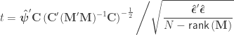
$t = \boldsymbol{\hat{\psi}}'\mathbf{C} \left(\mathbf{C}'(\mathbf{M}'\mathbf{M})^{-1}\mathbf{C} \right)^{-\frac{1}{2}} \left/ \sqrt{\dfrac{\boldsymbol{\hat{\epsilon}}'\boldsymbol{\hat{\epsilon}}}{N-\mathsf{rank}\left(\mathbf{M}\right)}} \right.$

where the hat on $\boldsymbol{\hat{\psi}}$ and $\boldsymbol{\hat{\epsilon}}$ indicate that these are quantities estimated from the sample. If $\mathsf{rank}\left(\mathbf{C}\right) \geqslant 1$ , the F statistic can be obtained as:

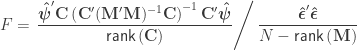
$F = \left.\dfrac{\boldsymbol{\hat{\psi}}'\mathbf{C} \left(\mathbf{C}'(\mathbf{M}'\mathbf{M})^{-1}\mathbf{C} \right)^{-1} \mathbf{C}'\boldsymbol{\hat{\psi}}}{\mathsf{rank}\left(\mathbf{C}\right)} \right/ \dfrac{\boldsymbol{\hat{\epsilon}}'\boldsymbol{\hat{\epsilon}}}{N-\mathsf{rank}\left(\mathbf{M}\right)}$

When $\mathsf{rank}\left(\mathbf{C}\right) = 1$ , $F = t^2$ . For either of these statistics, we can assess their significance by repeating the same fit after permuting $\mathbf{Y}$ or $\mathbf{M}$ (i.e., a permutation test), or by referring to the formula for the distribution of the corresponding statistic, which is available in most statistical software packages (i.e., a parametric test).

Permutation tests don’t depend on the same assumptions on which parametric tests are based. As some of these assumptions can be quite stringent in practice, permutation methods arguably should be preferred as a general framework for the statistical analysis of imaging data. At each permutation, a new statistic is computed and used to build its empirical distribution from which the p-values are obtained. In practice it’s not necessary to build the full distribution, and it suffices to increment a counter at each permutation. At the end, the counter is divided by the number of permutations to produce a p-value.

An example of a permutation distribution

Using permutation tests, correction for multiple testing using the family-wise error rate (fwer) is trivial: rather than build the permutation distribution at each voxel, a single distribution of the global maximum of the statistic across the image is constructed. Each permutation yields one maximum, that is used to build the distribution. Any dependence between the tests is implicitly captured, with not need to model it explicitly, nor to introduce even more assumptions, a problem that hinders methods such as the random field theory.

Exchangeability blocks

Permutation is allowed if it doesn’t affect the joint distribution of the error terms, i.e., if the errors are exchangeable. Some types of experiments may involve repeated measurements or other kinds of dependency, such that exchangeability cannot be guaranteed between all observations. However, various cases of structured dependency can still be accommodated if sets (blocks) of observations are shuffled as a whole, or if shuffling happens only within set (block). It is not necessary to know or to model the exact dependence structure between observations, which is captured implicitly as long as the blocks are defined correctly.

Permutation within block.

Permutation of blocks as a whole.

The two figures above are of designs constructed using the fsl software package. In fsl, within-block permutation is available in randomise with the option -e, used to supply a file with the definition of blocks. For whole-block permutation, in addition to the option -e, the option --permuteBlocks needs to be supplied.

The G-statistic

The presence of exchangeability blocks solves a problem, but creates another. Having blocks implies that observations may not be pooled together to produce a non-linear parameter estimate such as the variance. In other words: the mere presence of exchangeability blocks, either for shuffling within or as a whole, implies that the variances may not be the same across all observations, and a single estimate of this variance is likely to be inaccurate whenever the variances truly differ, or if the groups don’t have the same size. This also means that the F or t statistics may not behave as expected.

The solution is to use the block definitions and the permutation strategy is to define groups of observations that are known or assumed to have identical variances, and pool only the observations within group for variance estimation, i.e., to define variance groups (vgs).

The F-statistic, however, doesn’t allow such multiple groups of variances, and we need to resort to another statistic. In Winkler et al. (2014) we propose:

$G = \dfrac{\boldsymbol{\hat{\psi}}'\mathbf{C} \left(\mathbf{C}'(\mathbf{M}'\mathbf{W}\mathbf{M})^{-1}\mathbf{C} \right)^{-1} \mathbf{C}'\boldsymbol{\hat{\psi}}}{\Lambda \cdot s}$

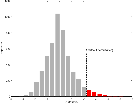
where $\mathbf{W}$ is a diagonal matrix that has elements:

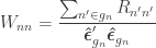
$W_{nn}=\dfrac{\sum_{n' \in g_{n}}R_{n'n'}}{\boldsymbol{\hat{\epsilon}}_{g_{n}}'\boldsymbol{\hat{\epsilon}}_{g_{n}}}$

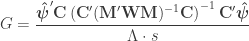
and where $R_{n'n'}$ are the $n'$ diagonal elements of the residual forming matrix, and $g_{n}$ is the variance group to which the $n$ -th observation belongs. The remaining denominator term, $\Lambda$ , is given by (Welch, 1951):

$\Lambda = 1+\frac{2(s-1)}{s(s+2)}\sum_{g} \frac{1}{\sum_{n \in g}R_{nn}} \left(1-\frac{\sum_{n \in g}W_{nn}}{\mathsf{trace}\left(\mathbf{W}\right)}\right)^2$

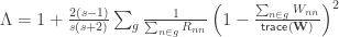
where $s=\mathsf{rank}\left(\mathbf{C}\right)$ . The matrix $\mathbf{W}$ can be seen as a weighting matrix, the square root of which normalises the model such that the errors have then unit variance and can be ignored. It can also be seen as being itself a variance estimator. In fact, it is the very same variance estimator proposed by Horn et al (1975).

The W matrix used with the G statistic. It is constructed from the estimated variances of the error terms.

The matrix $\mathbf{W}$ has a crucial role in making the statistic pivotal in the presence of heteroscedasticity. Pivotality means that the statistic has a sampling distribution that is not dependent on any unknown parameter. For imaging experiments, it’s important that the statistic has this property, otherwise correction for multiple testing that controls fwer will be inaccurate, or possibly invalid altogether.

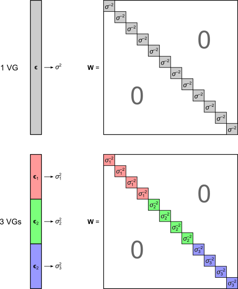
When $\mathsf{rank}\left(\mathbf{C}\right)=1$ , the t-equivalent to the G-statistic is 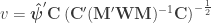$v = \boldsymbol{\hat{\psi}}'\mathbf{C} \left(\mathbf{C}'(\mathbf{M}'\mathbf{W}\mathbf{M})^{-1}\mathbf{C} \right)^{-\frac{1}{2}}$ , which is the well known Aspin-Welch $v$ -statistic for the Behrens-Fisher problem. The relationship between $v$ and G is the same as between t and F, i.e., when the rank of the contrast equals to one, the latter is simply the square of the former. The G statistic is a generalization of all these, and more, as we show in the paper, and summarise in the table below:

	$\mathsf{rank}\left(\mathbf{C}\right) = 1$	$\mathsf{rank}\left(\mathbf{C}\right) > 1$
Homoscedastic errors, unrestricted exchangeability	Square of Student’s t	F-ratio
Homoscedastic within vg, restricted exchangeability	Square of Aspin-Welch $v$	Welch’s $v^2$

In the absence of variance groups (i.e., all observations belong to the same vg), G and $v$ are equivalent to F and t respectively.

Although not typically necessary if permutation methods are to be preferred, approximate parametric p-values for the G-statistic can be computed from an F-distribution with $\nu_1=s$ and $\nu_2=2(s-1)/3/(\Lambda-1)$ .

While the error rates are controlled adequately (a feature of permutation tests in general), the G-statistic offers excellent power when compared to the F-statistic, even when the assumptions of the latter are perfectly met. Moreover, by preserving pivotality, it is an adequate statistic to control of the error rate in the in the presence of multiple tests.

In this post, the focus is in using G for imaging data, but of course, it can be used for any dataset in which a linear model where variances cannot be assumed to be the same is used, i.e., when heteroscedasticity is or could be present.

Note that the G-statistic has nothing to do with the G-test. It is named as this for being a generalisation over various tests, including the commonly used t and F tests, as shown above.