November | 2012 | Brainder.

Estimating the empirical cumulative distribution function (empirical cdf) from a set of observed values requires computing, for each value, how many of the other values are smaller or equal to it. In other words, let $X = \{x_1, x_2, \ldots , x_N\}$ be the observed values, then:

$F(x) = P(X \leqslant x) = \frac{1}{N} \sum_{n=1}^{N}I(x_n \leqslant x)$

where $F(x)$ is the empirical cdf, $P(X \leqslant x)$ is the probability of observing a value in $X$ that is smaller than or equal to $x$ , $I(\cdot)$ is a function that evaluates as 1 if the condition in the parenthesis is satisfied or 0 otherwise, and $N$ is the number of observations. This definition is straightforward and can be found in many statistical textbooks (see, e.g., Papoulis, 1991).

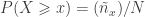
For continuous distributions, a p-value for a given $x \in X$ can be computed as $1-F(x)$ . For a discrete cdf, however, this trivial relationship does not hold. The reason is that, while for continuous distributions the probability $P(X = x) = 0$ , for discrete distributions (such as empirical distributions), $P(X = x) > 0$ whenever $x \in X$ . As we often want to assign a probability to one of the values that have been observed, the condition $x \in X$ always holds, and the simple relationship between the cdf and the p-value is lost. The solution, however, is still simple: a p-value can be obtained from the cdf as $1-F(x) + 1/N$ .

In the absence of repeated values (ties), the cdf can be obtained computationally by sorting the observed data in ascending order, i.e., $X_{s} = \{x_{(1)}, x_{(2)}, \ldots , x_{(N)}\}$ . Then $F(x)=(n_x)/N$ , where $(n_x)$ represents the ascending rank of $x$ . Likewise, the p-value can be obtaining by sorting the data in descending order, and using a similar formula, $P(X \geqslant x) = (\tilde{n}_x)/N$ , where $(\tilde{n}_x)$ represents the descending rank of $x$ .

Example 1: Consider the following sequence of 10 observed values, already sorted in ascending order:

$X=\{75, 76, 79, 80, 84, 85, 86, 88, 90, 94\}$

The corresponding ranks are simply 1, 2, 3, 4, 5, 6, 7, 8, 9, 10. Consequently, the cdf is:

$F(x|x\in X) = \{0.1, 0.2, 0.3, 0.4, 0.5, 0.6, 0.7, 0.8, 0.9, 1\}$

The p-values are computed by using the ranks in descending order, i.e., 10, 9, 8, 7, 6, 5, 4, 3, 2, 1, which yields:

$P(X \geqslant x | x \in X) = \{1, 0.9, 0.8, 0.7, 0.6, 0.5, 0.4, 0.3, 0.2, 0.1\}$

The problem with ties

Simple sorting, as above, is effective when there are no repeated values in the data. However, in the presence of ties, simple sorting that produces ordinal rankings yield incorrect results.

Example 2: Consider the following sequence of 10 observed values, in which ties are present:

$X = \{81, 81, 82, 83, 83, 83, 84, 85, 85, 85\}$

If the same computational strategy discussed above were used, the we would conclude that the p-value for $x=85$ would be either 0.1, 0.2 or 0.3, depending on which instance of the “85” we were to choose. The correct value, however, is 0.3 (only), since 3 out of 10 variables are equal or above 85. The solution to this problem is to replace the simple, ordinal ranking, for a modified version of the so called competition ranking.

The competition ranking

The competition ranking assigns the same rank to values that are identical. The standard competition ranking for the previous sequence is, in ascending order, 1, 1, 3, 4, 4, 4, 7, 8, 8, 8. In descending order, the ranks are 9, 9, 8, 5, 5, 5, 4, 1, 1, 1. Note that in this ranking, the ties receive the “best” possible rank. A slightly different approach consists in assigning the “worst” possible rank to the ties. This modified competition ranking applied the previous sequence gives, in ascending order, the ranks 2, 2, 3, 5, 5, 5, 7, 10, 10, 10, whereas in descending order, the ranks are 10, 10, 8, 7, 7, 7, 4, 3, 3, 3.

Competition ranking solves the problem with ties for both the empirical cdf and for the calculation of the p-values. In both cases, it is the modified version of the ranking that needs to be used, i.e., the ranking that assigns the worst rank to identical values. Still using the same sequence as example, the cdf is given by:

$F(x|x\in X) = \{0.2, 0.2, 0.3, 0.6, 0.6, 0.6, 0.7, 1, 1, 1\}$

and the p-values are given by:

$P(X \geqslant x | x \in X) = \{1, 1, 0.8, 0.7, 0.7, 0.7, 0.4, 0.3, 0.3, 0.3\}$

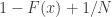
Note that, as in the case with no ties, the p-values cannot be computed simply as $1-F(x)$ from the cdf as it would for continuous distributions. The correct formula is $1-F(x)+(n_x)/N$ , with $(n_x)$ here representing the frequency of $x$ .

Uses

The cdf of a set of observed data is useful in many types of non-parametric inference, particularly those that use bootstrap, jack-knife, Monte Carlo, or permutation tests. Ties can be quite common when working with discrete data and discrete explanatory variables using any of these methods.

References

Papoulis A. Probability, Random Variables and Stochastic Processes. McGraw-Hill, New York, 3rd ed, 1991.