The lady tasting tea experiment

Posted on 23.August.2015 by A. M. Winkler

Can you tell?

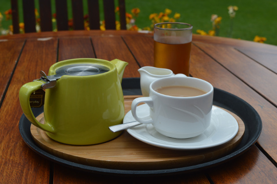
The now famous story is that in an otherwise unremarkable summer afternoon in Cambridge in the 1920’s, a group of friends eventually discussed about the claims made by one of the presents about her abilities on discriminating whether milk was poured first or last when preparing a cup of tea with milk. One of the presents was Ronald Fisher, and the story, along with a detailed description of how to conduct a simple experiment to test the claimed ability, and how to obtain an exact solution, was presented at length in the Chapter 2 of his book The Design of Experiments, a few lines of which are quoted below:

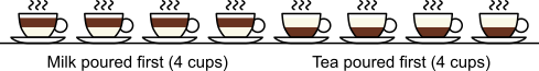
A lady declares that by tasting a cup of tea made with milk she can discriminate whether the milk or the tea infusion was first added to the cup. We will consider the problem of designing an experiment by means of which this assertion can be tested. […] [It] consists in mixing eight cups of tea, four in one way and four in the other, and presenting them to the subject for judgment in a random order. The subject has been told in advance of that the test will consist, namely, that she will be asked to taste eight cups, that these shall be four of each kind […]. — Fisher, 1935.

There are $\frac{8!}{4!4!}=70$ distinct possible orderings of these cups, and by telling the subject in advance that there are four cups of each type, this guarantees that the answer will include four of each.

The lady in question eventually answered correctly six out of the eight trials. The results can be assembled in a 2 by 2 contingency table:

		True order:		Total (margin)
		Tea first	Milk first	Total (margin)
Lady’s Guesses:	Tea first	$a=3$	$b=1$	$a+b=4$
Lady’s Guesses:	Milk first	$c=1$	$d=3$	$c+d=4$
Total (margin)		$a+c=4$	$b+d=4$	$n=8$

With these results, what should be concluded about the ability of the lady in discriminating whether milk or tea was poured first? It is not possible to prove that she would never be wrong, because if a sufficiently large number of cups of tea were offered, a single failure would disprove such hypothesis. However, a test that she is never right can be disproven, with a certain margin of uncertainty, given the number of cups offered.

Solution using Fisher’s exact method

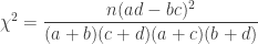
Fisher presented an exact solution for this experiment. It is exact in the sense that it allows an exact probability to be assigned to each of the possible outcomes. The probability can be calculated as:

$P_{\text{Fisher}} = \dfrac{(a+b)!(c+d)!(a+c)!(b+d)!}{n!a!b!c!d!}$

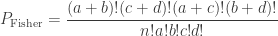
For the particular configuration of the contingency table above, the probability is $\frac{16}{70} = 0.22857$ . This is not the final result, though: what matters to disprove the hypothesis that she is not able to discriminate is how likely it would be for her to find a result at least as extreme as the one observed. In this case, there is one case that is more extreme, which would be the one in which she would have made correct guesses for all the 8 cups, in which case the values in the contingency table above would have been $a = 4$ , $b = 0$ , $c = 0$ , and $d = 4$ , with a probability computed with the same formula as $\frac{1}{70} = 0.01429$ . Adding these two probabilities together yield $\frac{16+1}{70}=0.24286$ .

Thus, if the lady is not able to discriminate whether tea or milk was poured first, the chance of observing a result at least as favourable towards her claim would be 0.24286, i.e., about 24%.

If from the outset we were willing to consider a significance level 0.05 (5%) as an informal rule to disprove the null hypothesis, we would have considered the p-value = 0.24286 as non-significant. This p-value is exact, a point that will become more clear below, in the section about permutation tests.

Using the hypergeometric distribution directly

The above process can become laborious for experiments with larger number of trials. An alternative, but equivalent solution, is to appeal directly to the hypergeometric distribution. The probability mass function (pmf) of this distribution can be written as a function the parameters of the contingency table as:

$P(X=a) = \dfrac{\binom{a+b}{a}\binom{c+d}{c}}{\binom{n}{a+c}}$

The pmf is equivalent to Fisher’s exact formula to compute the probability of a particular configuration. The cumulative density function, which is conditional on the margins being fixed, is:

$P(X \geqslant a) = \sum_{j=a}^{J}\dfrac{\binom{a+b}{j}\binom{c+d}{a+c-j}}{\binom{n}{a+c}} = \sum_{j=a}^{J}\dfrac{(a+b)!(c+d)!(a+c)!(b+d)!}{n!j!(a+b-j)!(a+c-j)!(d-a+j)!}$

where $J=\min(a+c,a+b)$ . Computing from the above (details omitted), yield the same value as using Fisher’s presentation, that is, the p-value is (exactly) 0.24286.

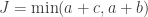
Solution using Pearson’s $\chi^2$ method

Much earlier than the tea situation described above, Karl Pearson had already considered the problem of inference in contingency tables, having proposed a test based on a $\chi^2$ statistic.

$\chi^2 = \sum_{i=1}^{R}\sum_{j=1}^{C}\dfrac{(O_{ij}-E_{ij})^2}{E_{ij}}$

where $O_{ij}$ is the observed value for the element in the position $(i,j)$ in the table, $R$ and $C$ are respectively the number of rows and columns, and $E_{ij}$ is the expected value for these elements if the null hypothesis is true. The values $E_{ij}$ can be computed as the product of the marginals for row $i$ and column $j$ , divided by the overall number of observations $n$ . A simpler, equivalent formula is given by:

$\chi^2 = \dfrac{n(ad - bc)^2}{(a+b)(c+d)(a+c)(b+d)}$

A p-value can be computed from the 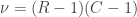$\chi^2$ distribution with degrees of freedom $\nu=(R-1)(C-1)$ .

Under the null, we can expect a value equal to 2 in each of the 2 cells, that is, the lady would for each cup have a 50:50 chance of answering correctly. For the original tea tasting experiment, Pearson’s method give quite inaccurate results: $\chi^2=2$ , which corresponds to a p-value of 0.07865. However, it is well known that this method is inaccurate if cells in the table have too small quantities, usually below 5 or 6.

Improvement using Yates’ continuity correction

To solve the above well-known issue with small quantities, Yates (1934) proposed a correction, such that the test statistic becomes:

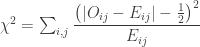
$\chi^2 = \sum_{i,j}\dfrac{\left(|O_{ij}-E_{ij}|-\frac{1}{2}\right)^2}{E_{ij}}$

Applying this correction to the original tea experiment gives $\chi^2=0.5$ , and a p-value of 0.23975, which is very similar to the one given by the Fisher method. Note again that this approach, like the $\chi^2$ test, predates Fisher’s exact test.

Equivalence of Fisher’s exact test and permutation tests

The method proposed by Fisher corresponds to a permutation test. Let $\mathbf{x}$ be a column vector containing binary indicators for whether milk was truly poured first. Let $\mathbf{y}$ be a column vector containing binary indicators for whether the lady answered that milk was poured first. The general linear model (GLM) can be used as usual, such that $\mathbf{y}=\mathbf{x}\beta + \boldsymbol{\epsilon}$ , where $\beta$ is a regression coefficient, and $\boldsymbol{\epsilon}$ are the residuals.

Under the null hypothesis that the lady cannot discriminate, the binary values in $\mathbf{y}$ can be permuted randomly. There are $\binom{8}{4}=70$ possible unique rearrangements. Out of these, in 17, there are 6 or more (out of 8) correct answers matching the values in $\mathbf{x}$ , which gives a p-value 17/70 = 0.24286.

Note that the strategy using the GLM can be used even if both variables $\mathbf{x}$ and $\mathbf{y}$ are binary, as in the example of the tea tasting, even if the residuals are not normally distributed (permutation tests do not depend on distributional assumptions), and even considering that values in $\beta$ can lead to non-sensical predictions in $\mathbf{y}$ , as prediction is not the objective of this analysis.

Why not a binomial test?

The binomial test could be considered if the lady did not know in advance that there were 4 cups of each mixture order. Since she knew (so the two margins of the table are fixed), each cup was not independent from each other, and her possible answers had to be constrained by answers previously given. The binomial test assumes independence, thus, is not an option for this analysis.

Relevance

Using this simple experiment, Fisher established most of the fundamental principles for hypothesis testing, which contributed to major advances across biological and physical sciences. A careful read of the original text shows a precise use of terms, in a concise and unambiguous presentation, in contrast with many later and more verbose textbooks that eventually hid from readers most of the fundamental principles.

References

Fisher, R. A. The Design of Experiments. Oliver and Boyd, Edinburgh, 1935.
Pearson K. X. On the criterion that a given system of deviations from the probable in the case of a correlated system of variables is such that it can be reasonably supposed to have arisen from random sampling. Philos Mag Ser 5. 1900 Jul;50(302):157–75.
Yates F. Contingency Tables Involving Small Numbers and the Chi^2 test. Suppl to J R Stat Soc. 1934;1(2):217–35.

The photograph at the top (tea with milk) is in public domain.

Variance components in genetic analyses

Posted on 02.August.2015 by A. M. Winkler

Pedigree-based analyses allow investigation of genetic and environmental influences on anatomy, physiology, and behaviour.

Methods based on components of variance have been used extensively to assess genetic influences and identify loci associated with various traits quantifying aspects of anatomy, physiology, and behaviour, in both normal and pathological conditions. In an earlier post, indices of genetic resemblance between relatives were presented, and in the last post, the kinship matrix was defined. In this post, these topics are used to present a basic model that allows partitioning of the phenotypic variance into sources of variation that can be ascribed to genetic, environmental, and other factors.

A simple model

Consider the model:

$\mathbf{Y} = \mathbf{X}\mathbf{B} + \boldsymbol{\Upsilon}$

where, for $S$ subjects, $T$ traits, $P$ covariates and $K$ variance components, $\mathbf{Y}_{S \times T}$ are the observed trait values for each subject, $\mathbf{X}_{S \times P}$ is a matrix of covariates, $\mathbf{B}_{P \times T}$ is a matrix of unknown covariates’ weights, and $\boldsymbol{\Upsilon}_{S \times T}$ are the residuals after the covariates have been taken into account.

The elements of each column $t$ of $\boldsymbol{\Upsilon}$ are assumed to follow a multivariate normal distribution $\mathcal{N}\left(0;\mathbf{S}\right)$ , where $\mathbf{S}$ is the between-subject covariance matrix. The elements of each row $s$ of $\boldsymbol{\Upsilon}$ are assumed to follow a normal distribution $\mathcal{N}\left(0;\mathbf{R}\right)$ , where $\mathbf{R}$ is the between-trait covariance matrix. Both $\mathbf{R}$ and $\mathbf{S}$ are seen as the sum of $K$ variance components, i.e. $\mathbf{R} = \sum_{k} \mathbf{R}_{k}$ and $\mathbf{S} = \sum_{k} \mathbf{S}_{k}$ . For a discussion on these equalities, see Eisenhart (1947) [see references at the end].

An equivalent model

The same model can be written in an alternative way. Let $\mathbf{y}_{S \cdot T \times 1}$ be the stacked vector of traits, $\mathbf{\tilde{X}}_{S \cdot T \times P \cdot T} = \mathbf{X} \otimes \mathbf{I}_{T \times T}$ is the matrix of covariates, $\boldsymbol{\beta}_{P \cdot T \times 1}$ the vector with the covariates’ weights, $\boldsymbol{\upsilon}_{S \cdot T \times 1}$ the residuals after the covariates have been taken into account, and $\otimes$ represent the Kronecker product. The model can then be written as:

$\mathbf{y} = \mathbf{\tilde{X}}\boldsymbol{\beta} + \boldsymbol{\upsilon}$

The stacked residuals $\boldsymbol{\upsilon}$ is assumed to follow a multivariate normal distribution $\mathcal{N}\left(0;\boldsymbol{\Omega}\right)$ , where $\boldsymbol{\Omega}$ can be seen as the sum of $K$ variance components:

$\boldsymbol{\Omega} = \sum_{k} \mathbf{R}_k \otimes \mathbf{S}_k$

The $\boldsymbol{\Omega}$ here is the same as in Almasy and Blangero (1998). $\mathbf{S}_k$ can be modelled as correlation matrices. The associated scalars are absorbed into the (to be estimated) $\mathbf{R}_k$ . $\mathbf{R}$ is the phenotypic covariance matrix between the residuals of the traits:

$\mathbf{R} = \left[ \begin{array}{ccc} \mathsf{Var}(\upsilon_1) & \cdots & \mathsf{Cov}(\upsilon_1,\upsilon_T) \\ \vdots & \ddots & \vdots \\ \mathsf{Cov}(\upsilon_T,\upsilon_1) & \cdots & \mathsf{Var}(\upsilon_T) \end{array}\right]$

whereas each $\mathbf{R}_k$ are the share of these covariances attributable to the $k$ -th component:

$\mathbf{R}_k = \left[ \begin{array}{ccccc} \mathsf{Var}_k(\upsilon_1) & \cdots & \mathsf{Cov}_k(\upsilon_1,\upsilon_T) \\ \vdots & \ddots & \vdots \\ \mathsf{Cov}_k(\upsilon_T,\upsilon_1) & \cdots & \mathsf{Var}_k(\upsilon_T) \end{array}\right]$

$\mathbf{R}$ can be converted to a between-trait phenotypic correlation matrix $\mathbf{\mathring{R}}$ as:

$\mathbf{\mathring{R}} = \left[ \begin{array}{ccc} \frac{\mathsf{Var}(\upsilon_1)}{\mathsf{Var}(\upsilon_1)} & \cdots & \frac{\mathsf{Cov}(\upsilon_1,\upsilon_T)}{\left(\mathsf{Var}(\upsilon_1)\mathsf{Var}(\upsilon_T)\right)^{1/2}} \\ \vdots & \ddots & \vdots \\ \frac{\mathsf{Cov}(\upsilon_1,\upsilon_T)}{\left(\mathsf{Var}(\upsilon_1)\mathsf{Var}(\upsilon_T)\right)^{1/2}} & \cdots & \frac{\mathsf{Var}(\upsilon_T)}{\mathsf{Var}(\upsilon_T)} \end{array}\right]$

The above phenotypic correlation matrix has unit diagonal and can still be fractioned into their $K$ components:

$\mathbf{\mathring{R}}_k = \left[ \begin{array}{ccc} \frac{\mathsf{Var}_k(\upsilon_1)}{\mathsf{Var}(\upsilon_1)} & \cdots & \frac{\mathsf{Cov}_k(\upsilon_1,\upsilon_T)}{\left(\mathsf{Var}(\upsilon_1)\mathsf{Var}(\upsilon_T)\right)^{1/2}} \\ \vdots & \ddots & \vdots \\ \frac{\mathsf{Cov}_k(\upsilon_T,\upsilon_1)}{\left(\mathsf{Var}(\upsilon_T)\mathsf{Var}(\upsilon_1)\right)^{1/2}} & \cdots & \frac{\mathsf{Var}_k(\upsilon_T)}{\mathsf{Var}(\upsilon_T)} \end{array}\right]$

The relationship $\mathbf{\mathring{R}} = \sum_k \mathbf{\mathring{R}}_k$ holds. The diagonal elements of $\mathbf{\mathring{R}}_k$ may receive particular names, e.g., heritability, environmentability, dominance effects, shared enviromental effects, etc., depending on what is modelled in the corresponding $\mathbf{S}_k$ . However, the off-diagonal elements of $\mathbf{\mathring{R}}_k$ are not the $\rho_k$ that correspond, e.g. to the genetic or environmental correlation. These off-diagonal elements are instead the signed $\text{\textsc{erv}}$ when $\mathbf{S}_k=2\cdot\boldsymbol{\Phi}$ , or their $\text{\textsc{erv}}_k$ -equivalent for other variance components (see below). In this particular case, they can also be called “bivariate heritabilities” (Falconer and MacKay, 1996). A matrix $\mathbf{\breve{R}}_k$ that contains these correlations $\rho_k$ , which are the fraction of the variance attributable to the $k$ -th component that is shared between pairs of traits is given by:

$\mathbf{\breve{R}}_k = \left[ \begin{array}{ccc} \frac{\mathsf{Var}_k(\upsilon_1)}{\mathsf{Var}_k(\upsilon_1)} & \cdots & \frac{\mathsf{Cov}_k(\upsilon_1,\upsilon_T)}{\left(\mathsf{Var}_k(\upsilon_1)\mathsf{Var}_k(\upsilon_T)\right)^{1/2}} \\ \vdots & \ddots & \vdots \\ \frac{\mathsf{Cov}_k(\upsilon_T,\upsilon_1)}{\left(\mathsf{Var}_k(\upsilon_T)\mathsf{Var}_k(\upsilon_1)\right)^{1/2}} & \cdots & \frac{\mathsf{Var}_k(\upsilon_T)}{\mathsf{Var}_k(\upsilon_T)} \end{array}\right]$

As for the phenotypic correlation matrix, each $\mathbf{\breve{R}}_k$ has unit diagonal.

The most common case

A particular case is when $\mathbf{S}_1 = 2\cdot\boldsymbol{\Phi}$ , the coefficient of familial relationship between subjects, and $\mathbf{S}_2 = \mathbf{I}_{S \times S}$ . In this case, the $T$ diagonal elements of $\mathbf{\mathring{R}}_1$ represent the heritability ( $h_t^2$ ) for each trait $t$ . The diagonal of $\mathbf{\mathring{R}}_2$ contains $1-h_t^2$ , the environmentability. The off-diagonal elements of $\mathbf{\mathring{R}}_1$ contain the signed $\text{\textsc{erv}}$ (see below). The genetic correlations, $\rho_g$ are the off-diagonal elements of $\mathbf{\breve{R}}_1$ , whereas the off-diagonal elements of $\mathbf{\breve{R}}_2$ are $\rho_e$ , the environmental correlations between traits. In this particular case, the components of $\mathbf{R}$ , i.e., $\mathbf{R}_k$ are equivalent to $\mathbf{G}$ and $\mathbf{E}$ covariance matrices as in Almasy et al (1997).

Relationship with the ERV

To see how the off-diagonal elements of $\mathbf{\mathring{R}}_k$ are the signed Endophenotypic Ranking Values for each of the $k$ -th variance component, $\text{\textsc{erv}}_k$ (Glahn et al, 2011), note that for a pair of traits $i$ and $j$ :

$\mathring{R}_{kij} = \frac{\mathsf{Cov}_k(\upsilon_i,\upsilon_j)}{\left(\mathsf{Var}(\upsilon_i)\mathsf{Var}(\upsilon_j)\right)^{1/2}}$

Multiplying both numerator and denominator by $\left(\mathsf{Var}_k(\upsilon_i)\mathsf{Var}_k(\upsilon_j)\right)^{1/2}$ and rearranging the terms gives:

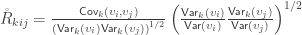
$\mathring{R}_{kij} = \frac{\mathsf{Cov}_k(\upsilon_i,\upsilon_j)}{\left(\mathsf{Var}_k(\upsilon_i)\mathsf{Var}_k(\upsilon_j)\right)^{1/2}} \left(\frac{\mathsf{Var}_k(\upsilon_i)}{\mathsf{Var}(\upsilon_i)}\frac{\mathsf{Var}_k(\upsilon_j)}{\mathsf{Var}(\upsilon_j)}\right)^{1/2}$

When $\mathbf{S}_k = 2\cdot\boldsymbol{\Phi}$ , the above reduces to $\mathring{R}_{kij} = \rho_k \sqrt{h^2_i h^2_j}$ , which is the signed version of $\text{\textsc{erv}}=\left|\rho_g\sqrt{h_i^2h_j^2}\right|$ when $k$ is the genetic component.

Positive-definiteness

$\mathbf{R}$ and $\mathbf{R}_k$ are covariance matrices and so, are positive-definite, whereas the correlation matrices $\mathbf{\mathring{R}}$ , $\mathbf{\mathring{R}}_k$ and $\mathbf{\breve{R}}_k$ are positive-semidefinite. A hybrid matrix that does not have to be positive-definite or semidefinite is:

$\mathbf{\check{R}}_k = \mathbf{I} \odot \mathbf{\mathring{R}}_k + \left(\mathbf{J}-\mathbf{I}\right) \odot \mathbf{\breve{R}}_k$

where $\mathbf{J}$ is a matrix of ones, $\mathbf{I}$ is the identity, both of size $T \times T$ , and $\odot$ is the Hadamard product. An example of such matrix of practical use is to show concisely the heritabilities for each trait in the diagonal and the genetic correlations in the off-diagonal.

Cauchy-Schwarz

Algorithmic advantages can be obtained from the positive-definiteness of $\mathbf{\mathring{R}}_k$ . The Cauchy–Schwarz theorem (Cauchy, 1821; Schwarz, 1888) states that:

$\mathring{R}_{kij} \leqslant \sqrt{\mathring{R}_{kii}\mathring{R}_{kjj}}$

Hence, the bounds for the off-diagonal elements can be known from the diagonal elements, which, by their turn, are estimated in a simpler, univariate model.

The Cauchy-Schwarz inequality imposes limits on the off-diagonal values of the matrix that contains the genetic covariances (or bivariate heritabilities).

Parameter estimation

Under the multivariate normal assumption, the parameters can be estimated maximising the following loglikelihood function:

$\mathcal{L}\left(\mathbf{R}_k,\boldsymbol{\beta}\Big|\mathbf{y},\mathbf{\tilde{X}}\right) = -\frac{1}{2} \left(N \ln 2\pi + \ln \left|\boldsymbol{\Omega}\right| + \left(\mathbf{y}-\mathbf{\tilde{X}}\boldsymbol{\beta}\right)'\boldsymbol{\Omega}\left(\mathbf{y}-\mathbf{\tilde{X}}\boldsymbol{\beta}\right)\right)$

where $N=S \cdot T$ is the number of observations on the stacked vector $\mathbf{y}$ . Unbiased estimates for $\boldsymbol{\beta}$ , although inefficient and inappropriate for hypothesis testing, can be obtained with ordinary least squares (OLS).

Parametric inference

Hypothesis testing can be performed with the likelihood ratio test (LRT), i.e., the test statistic is produced by subtracting from the loglikelihood of the model in which all the parameters are free to vary ( $\mathcal{L}_1$ ), the loglikelihood of a model in which the parameters being tested are constrained to zero, the null model ( $\mathcal{L}_0$ ). The statistic is given by $\lambda = 2\left(\mathcal{L}_1-\mathcal{L}_0\right)$ (Wilks, 1938), which here is asymptotically distributed as a 50:50 mixture of a $\chi^2_0$ and $\chi^2_{\text{df}}$ distributions, where df is the number of parameters being tested and free to vary in the unconstrained model (Self and Liang, 1987). From this distribution the p-values can be obtained.