A higher Octave for PALM

Posted on 08.October.2019 by A. M. Winkler

PALM — Pemutation Analysis of Linear Models — uses either MATLAB or Octave behind the scenes. It can be executed from within either of these environments, or from the shell, in which case either of these is invoked, depending on how PALM was configured.

For users who do not want or cannot spend thousands of dollars in MATLAB licenses, Octave comes for free, and offers quite much the same benefits. However, for Octave, some functionalities in PALM require version 4.4.1 or higher. However, stable Linux distributions such as Red Hat Enterprise Linux and related (such as CentOS and Scientific Linux) still offer only 3.8.2 in the official repositories at the time of this writing, leaving the user with the task of finding an unofficial package or compiling from the source. The latter task, however, can be daunting: Octave is notoriously difficult to compile, with a myriad of dependencies.

A much simpler approach is to use Flatpak or Snappy. These are systems for distribution of Linux applications. Snappy is sponsored by Canonical (that maintains Ubuntu), whereas Flatpak appears to be the preferred tool for Fedora and openSUSE. Using either system is quite simple, and here the focus is on Flatpak.

To have a working installation of Octave, all that needs be done is:

1) Make sure Flatpak is installed:

On a RHEL/CentOS system, use (as root):

yum install flatpak

For openSUSE, use (as root):

zypper install flatpak

For Ubuntu and other Debian-based systems:

sudo apt install flatpak

2) Add the Flathub repository:

flatpak remote-add --if-not-exists flathub https://flathub.org/repo/flathub.flatpakrepo

3) Install Octave:

flatpak install flathub org.octave.Octave

4) Run it!

flatpak run org.octave.Octave

Only the installation of Flatpak needs be done as root. Once it has been installed, repositories and applications (such as Octave, among many others) can be installed at the user level. These can also be installed and made available system-wide (if run as root).

Configuring PALM

From version alpha117 onwards, the executable file ‘palm’ (not to be confused with ‘palm.m’) will include a variable named “OCTAVEBIN”, which specifies how Octave should be called. Change it from the default:

OCTAVEBIN=/usr/bin/octave

so that it invokes the version installed with Flatpak:

OCTAVEBIN="/usr/bin/flatpak run org.octave.Octave"

After making the above edits, it should be possible to run PALM directly from the system shell using the version installed via Flatpak. Alternatively, it should also be possible to invoke Octave (as in step 4 above), then use the command “addpath” to specify the location of palm.m, and then call PALM from the Octave prompt.

Octave packages

Handling of packages when Octave is installed via Flatpak is the same as usual, that is, via the command ‘pkg’ run from within Octave. More details here.

The “Group” indicator in FSL

Posted on 24.February.2017 by A. M. Winkler

In FSL, when we create a design using the graphical interface in FEAT, or with the command Glm, we are given the opportunity to define, at the higher-level, the “Group” to which each observation belongs. When the design is saved, the information from this setting is stored in a text file named something as “design.grp”. This file, and thus the group setting, takes different roles depending whether the analysis is used in FEAT itself, in PALM, or in randomise.

What can be confusing sometimes is that, in all three cases, the “Group” indicator does not refer to experimental or observational group of any sort. Instead, it refers to variance groups (VG) in FEAT, to exchangeability blocks (EB) in randomise, and to either VG or EB in PALM, depending on whether the file is supplied with the options -vg or -eb.

In FEAT, unless there is reason to suspect (or assume) that the variances for different observations are not equal, all subjects should belong to group “1”. If variance groups are defined, then these are taken into account when the variances are estimated. This is only possible if the design matrix is “separable”, that is, it must be such that, if the observations are sorted by group, the design can be constructed by direct sum (i.e., block-diagonal concatenation) of the design matrices for each group separately. A design is not separable if any explanatory variable (EV) present in the model crosses the group borders (see figure below). Contrasts, however, can encompass variables that are defined across multiple VGs.

The variance groups not necessarily must match the experimental observational groups that may exist in the design (for example, in a comparison of patients and controls, the variance groups may be formed based on the sex of the subjects, or another discrete variable, as opposed to the diagnostic category). Moreover, the variance groups can be defined even if all variables in the model are continuous.

In randomise, the same “Group” setting can be supplied with the option -e design.grp, thus defining exchangeability blocks. Observations within a block can only be permuted with other observations within that same block. If the option --permuteBlocks is also supplied, then the EBs must be of the same size, and the blocks as a whole are instead then permuted. Randomise does not use the concept of variance group, and all observations are always members of the same single VG.

In PALM, using -eb design.grp has the same effect that -e design.grp has in randomise. Further using the option -whole is equivalent to using --permuteBlocks in randomise. It is also possible to use together -whole and -within, meaning that the blocks as a whole are shuffled, and further, observations within block are be shuffled. In PALM the file supplied with the option -eb can have multiple columns, indicating multi-level exchangeability blocks, which are useful in designs with more complex dependence between observations. Using -vg design.grp causes PALM to use the v– or G-statistic, which are replacements for the t– and F-statistics respectively for the cases of heterogeneous variances. Although VG and EB are not the same thing, and may not always match each other, the VGs can be defined from the EBs, as exchangeability implies that some observations must have same variance, otherwise permutations are not possible. The option -vg auto defines the variance groups from the EBs, even for quite complicated cases.

In both FEAT and PALM, defining VGs will only make a difference if such variance groups are not balanced, i.e., do not have the same number of observations, since heteroscedasticity (different variances) only matter in these cases. If the groups have the same size, all subjects can be allocated to a single VG (e.g., all “1”).

Better statistics, faster

Posted on 09.August.2016 by A. M. Winkler

Faster permutation inference

Permutation tests are more robust and help to make scientific results more reproducible by depending on fewer assumptions. However, they are computationally intensive as recomputing a model thousands of times can be slow. The purpose of this post is to briefly list some options available for speeding up permutation.

Firstly, no speed-ups may be needed: for small sample sizes, or low resolutions, or small regions of interest, a permutation test can run in a matter of minutes. For larger data, however, accelerations may be of use. One option is acceleration through parallel processing or GPUs (for example applications of the latter, see Eklund et al., 2012, Eklund et al., 2013 and Hernández et al., 2013; references below), though this does require specialised implementation. Another option is to reduce the computational burden by exploiting the properties of the statistics and their distributions. A menu of options includes:

Do few permutations (shorthand name: fewperms). The results remain valid on average, although the p-values will have higher variability.
Keep permuting until a fixed number of permutations with statistic larger than the unpermuted is found (a.k.a., negative binomial; shorthand name: negbin).
Do a few permutations, then approximate the tail of the permutation distribution by fitting a generalised Pareto distribution to its tail (shorthand name: tail).
Approximate the permutation distribution with a gamma distribution, using simple properties of the test statistic itself, amazingly not requiring any permutations at all (shorthand name: noperm).
Do a few permutations, then approximate the full permutation distribution by fitting a gamma distribution (shorthand name: gamma).
Run permutations on only a few voxels, then fill the missing ones using low-rank matrix completion theory (shorthand name: lowrank).

These strategies allow accelerations >100x, yielding nearly identical results as in the non-accelerated case. Some, such as tail approximation, are generic enough to be used nearly all the most common scenarios, including univariate and multivariate tests, spatial statistics, and for correction for multiple testing.

In addition to accelerating permutation tests, some of these strategies, such as tail and noperm, allow continuous p-values to be found, and refine the p-values far into the tail of the distribution, thus avoiding the usual discreteness of p-values, which can be a problem in some applications if too few permutations are done.

These methods are available in the tool PALM — Permutation Analysis of Linear Models — and the complete description, evaluation, and application to the re-analysis of a voxel-based morphometry study (Douaud et al., 2007) have been just published in Winkler et al., 2016 (for the Supplementary Material, click here). The paper includes a flow chart prescribing these various approaches for each case, reproduced below.

The hope is that these accelerations will facilitate the use of permutation tests and, if used in combination with hardware and/or software improvements, can further expedite computation leaving little reason not to use these tests.

References

Douaud G, Smith S, Jenkinson M, Behrens T, Johansen-Berg H, Vickers J, James S, Voets N, Watkins K, Matthews PM, James A. Anatomically related grey and white matter abnormalities in adolescent-onset schizophrenia. Brain. 2007 Sep;130(Pt 9):2375-86. Epub 2007 Aug 13.
Eklund A, Andersson M, Knutsson H. fMRI analysis on the GPU-possibilities and challenges. Comput Methods Programs Biomed. 2012 Feb;105(2):145-61.
Eklund A, Dufort P, Forsberg D, LaConte SM. Medical image processing on the GPU – Past, present and future. Med Image Anal. 2013;17(8):1073-94.
Hernández M, Guerrero GD, Cecilia JM, García JM, Inuggi A, Jbabdi S, et al. Accelerating fibre orientation estimation from diffusion weighted magnetic resonance imaging using GPUs. PLoS One. 2013 Jan;8(4):e61892.1.
Winkler AM, Ridgway GR, Webster MA, Smith SM, Nichols TE. Permutation inference for the general linear model. Neuroimage. 2014 May 15;92:381-97.
Winkler AM, Ridgway GR, Douaud G, Nichols TE, Smith SM. Faster permutation inference in brain imaging. Neuroimage. 2016 Jun 7;141:502-516.

Contributed to this post: Tom Nichols, Ged Ridgway.

Three HCP utilities

Posted on 01.August.2016 by A. M. Winkler

If you are working with data from the Human Connectome Project (HCP), perhaps these three small Octave/MATLAB utilities may be of some use:

hcp2blocks.m: Takes the restricted file with information about kinship and zygosity and produces a multi-level exchangeability blocks file that can be used with PALM for permutation inference. It is fully described here.
hcp2solar.m: Takes restricted and unrestricted files to produce a pedigree file that can be used with SOLAR for heritability and genome-wide association analyses.
picktraits.m: Takes either restricted or unrestricted files, a list of traits and a list of subject IDs to produce tables with selected traits for the selected subjects. These can be used to, e.g., produce design matrices for subsequent analysis.

These functions need to parse relatively large CSV files, which is somewhat inefficient in MATLAB and Octave. Still, since these commands usually have to be executed only once for a particular analysis, a 1-2 minute wait seems acceptable.

If downloaded directly from the above links, remember also to download the prerequisites: strcsvread.m and strcsvwrite.m. Alternatively, clone the full repository from GitHub. The link is this. Other tools may be added in the future.

A fourth utility

For the HCP-S1200 release (March/2017), zygosity information is provided in the fields ZygositySR (self-reported zygosity) and ZygosityGT (zygosity determined by genetic methods for select subjects). If needed, these two fields can be merged into a new field named simply Zygosity. To do so, use a fourth utility, command mergezyg.

Extreme value notes

Posted on 01.March.2016 by A. M. Winkler

Extreme values are useful to quantify the risk of catastrophic floods, and much more.

This is a brief set of notes with an introduction to extreme value theory. For reviews, see Leadbetter et al (1983) and David and Huser (2015) [references at the end]. Also of some (historical) interest might be the classical book by Gumbel (1958). Let $X_1, \dots, X_n$ be a sequence of independent and identically distributed variables with cumulative distribution function (cdf) $F(x)$ and let $M_n =\max(X_1,\dots,X_n)$ denote the maximum.

If $F(x)$ is known, the distribution of the maximum is:

$\begin{array}{lll} P(M_n \leqslant x) &=&P(X_1 \leqslant x, \dots, X_n \leqslant x) \\ &=& P(X_1 \leqslant x) \cdots P(X_n \leqslant x) = F^n(x). \end{array}$

The distribution function $F(x)$ might, however, not be known. If data are available, it can be estimated, although small errors on the estimation of $F(x)$ can lead to large errors concerning the extreme values. Instead, an asymptotic result is given by the extremal types theorem, also known as Fisher-Tippett-Gnedenko Theorem, First Theorem of Extreme Values, or extreme value trinity theorem (called under the last name by Picklands III, 1975).

But before that, let’s make a small variable change. Working with $M_n$ directly is problematic because as $n \rightarrow \infty$ , $F^n(x) \rightarrow 0$ . Redefining the problem as a function of $M_n^* = \frac{M_n-b_n}{a_n}$ renders treatment simpler. The theorem can be stated then as: If there exist sequences of constants $a_n \in \mathbb{R}_{+}$ and $b_n \in \mathbb{R}$ such that, as $n \rightarrow \infty$ :

$P\left(M_{n}^{*} \leqslant x \right) \rightarrow G(x)$

then $G(x)$ belongs to one of three “domains of attraction”:

Type I (Gumbel law): $\Lambda(x) = e^{-e^{-\frac{x-b}{a}}}$ , for $x \in \mathbb{R}$ indicating that the distribution of $M_n$ has an exponential tail.
Type II (Fréchet law): $\Phi(x) = \begin{cases} 0 & x\leqslant b \\ e^{-\left(\frac{x-b}{a}\right)^{-\alpha}} & x\; \textgreater\; b \end{cases}$ indicating that the distribution of $M_n$ has a heavy tail (including polynomial decay).
Type III (Weibull law): $\Psi(x) = \begin{cases} e^{-\left( -\frac{x-b}{a}\right)^\alpha} & x\;\textless\; b \\ 1 & x\geqslant b \end{cases}$ indicating that the distribution of $M_n$ has a light tail with finite upper bound.

Note that in the above formulation, the Weibull is reversed so that the distribution has an upper bound, as opposed to a lower one as in the Weibull distribution. Also, the parameterisation is slightly different than the one usually adopted for the Weibull distribution.

These three families have parameters $a\; \textgreater\; 0$ , $b$ and, for families II and III, $\alpha\; \textgreater\; 0$ . To which of the three a particular $F(x)$ is attracted is determined by the behaviour of the tail of of the distribution for large $x$ . Thus, we can infer about the asymptotic properties of the maximum while having only a limited knowledge of the properties of $F(x)$ .

These three limiting cases are collectively termed extreme value distributions. Types II and III were identified by Fréchet (1927), whereas type I was found by Fisher and Tippett (1928). In his work, Fréchet used $M_n^* = \frac{M_n}{a_n}$ , whereas Fisher and Tippett used $M_n^* = \frac{M_n-b_n}{a_n}$ . Von Mises (1936) identified various sufficient conditions for convergence to each of these forms, and Gnedenko (1943) established a complete generalisation.

Generalised extreme value distribution

As shown above, the rescaled maxima converge in distribution to one of three families. However, all are cases of a single family that can be represented as:

$G(x) = e^{-\left(1-\xi\left(\frac{x-\mu}{\sigma}\right)\right)^{\frac{1}{\xi}}}$

defined on the set $\left\{x:1-\xi\frac{x-\mu}{\sigma}\;\textgreater\;0\right\}$ , with parameters $-\infty \;\textless \;\mu\;\textless\; \infty$ (location), $\sigma\;\textgreater\;0$ (scale), and $-\infty\;\textless\;\xi\;\textless\;\infty$ (shape). This is the generalised extreme value (GEV) family of distributions. If $\xi \rightarrow 0$ , it converges to Gumbel (type I), whereas if $\xi < 0$ it corresponds to Fréchet (type II), and if $\xi\;\textgreater\;0$ it corresponds to Weibull (type III). Inference on $\xi$ allows choice of a particular family for a given problem.

Generalised Pareto distribution

For $u\rightarrow\infty$ , the limiting distribution of a random variable $Y=X-u$ , conditional on $X \;\textgreater\; u$ , is:

$H(y) = 1-\left(1-\frac{\xi y}{\tilde{\sigma}}\right)^{\frac{1}{\xi}}$

defined for $y \;\textgreater\; 0$ and $\left(1-\frac{\xi y}{\tilde{\sigma}}\right) \;\textgreater\; 0$ . The two parameters are the $\xi$ (shape) and $\tilde{\sigma}$ (scale). The shape corresponds to the same parameter $\xi$ of the GEV, whereas the scale relates to the scale of the former as $\tilde{\sigma}=\sigma-\xi(u-\mu)$ .

The above is sometimes called the Picklands-Baikema-de Haan theorem or the Second Theorem of Extreme Values, and it defines another family of distributions, known as generalised Pareto distribution (GPD). It generalises an exponential distribution with parameter $\frac{1}{\tilde{\sigma}}$ as $\xi \rightarrow 0$ , an uniform distribution in the interval $\left[0, \tilde{\sigma}\right]$ when $\xi = 1$ , and a Pareto distribution when $\xi \;\textgreater\; 0$ .

Parameter estimation

By restricting the attention to the most common case of $-\frac{1}{2}<\xi<\frac{1}{2}$ , which represent distributions approximately exponential, parametters for the GPD can be estimated using at least three methods: maximum likelihood, moments, and probability-weighted moments. These are described in Hosking and Wallis (1987). For $\xi$ outside this interval, methods have been discussed elsewhere (Oliveira, 1984). The method of moments is probably the simplest, fastest and, according to Hosking and Wallis (1987) and Knijnenburg et al (2009), has good performance for the typical cases of $-\frac{1}{2}<\xi<\frac{1}{2}$ .

For a set of extreme observations, let $\bar{x}$ and $s^2$ be respectively the sample mean and variance. The moment estimators of $\tilde{\sigma}$ and $\xi$ are $\hat{\tilde{\sigma}} = \frac{\bar{x}}{2}\left(\frac{\bar{x}^2}{s^2}+1\right)$ and $\hat{\xi}=\frac{1}{2}\left(\frac{\bar{x}^2}{s^2}-1\right)$ .

The accuracy of these estimates can be tested with, e.g., the Anderson-Darling goodness-of-fit test (Anderson and Darling, 1952; Choulakian and Stephens, 2001), based on the fact that, if the modelling is accurate, the p-values for the distribution should be uniformly distributed.

Availability

Statistics of extremes are used in PALM as a way to accelerate permutation tests. More details to follow soon.

References

Anderson TW, Darling DA. Asymptotic theory of certain goodness of fit criteria based on stochastic processes. Ann Math Stat. 1952;23(2):193-212.
Choulakian V, Stephens MA. Goodness-of-Fit Tests for the Generalized Pareto Distribution. Technometrics. 2001;43(4):478-84.
Davison AC, Huser R. Statistics of Extremes. Annu Rev Stat Its Appl. 2015;2(1):203-35.
Fisher RA, Tippett LHC. Limiting forms of the frequency distribution of the largest and smallest member of a sample. Proc Camb Philol Soc. 1928;24:180-90.
Fréchet, M. Sur la loi de probabilité de l’écart maximum. Ann Soc Polon Math. 1927;6:93. [link currently not accessible due to copyright issues]
Gnedenko B. Sur La Distribution Limite Du Terme Maximum D’Une Serie Aleatoire. Ann Math. 1943;44(3):423-53.
Gumbel E. Statistics of Extremes. Echo Point Books & Media, 1958.
Hosking JRM, Wallis JR. Parameter and quantile estimation for the generalized Pareto distribution. Technometrics. 1987;29:339-49.
Knijnenburg TA, Wessels LFA, Reinders MJT, Shmulevich I. Fewer permutations, more accurate P-values. Bioinformatics. 2009 Jun 15;25(12):i161-8.
Leadbetter MR, Lindgren G, Rootzén H. Extremes and related properties of
random sequences and processes. Springer-Verlag, New York, 1983.
Oliveira JT (ed). Proceedings of the NATO Advanced Study Institute on Statistical Extremes and Applications. D. Heidel, Dordrecht, Holland, 1984.
Picklands III J. Statistical inference using extreme order statistics. Ann Stat. 1975;3(1):119-31.
Tippett LHC. On the extreme individuals and the range of samples taken from a normal population. Biometrika. 1925;17(3):364-87.
von Mises R. La distribution de la plus grande de n valeurs. Rev Mathématique l’Union Interbalkanique. 1936;1:141-60.

The figure at the top (flood) is in public domain.

FSL on the Raspberry Pi

Posted on 23.December.2015 by A. M. Winkler

How about processing brain imaging data on a Raspberry Pi? The different versions of this little device have performed exceptionally well for education, entertainment, and for a variety of do-it-yourself projects, with many examples listed in websites such as Instructables and Adafruit. Most of these applications are not computationally as intensive. Yet, the small size, low power consumption, improved hardware in recent models, and low price, may make this feasible.

The Pi 2

Released earlier this year, the Raspberry Pi 2 (Model B) features a quad-core 900 MHz ARM processor, 1 GB of RAM, GPU, 4 USB ports, 10/100 Mbps Ethernet, HDMI and audio outputs, camera and display ports, as well as a low level general purpose interface (GPIO), all in a portable board of 85.6 mm × 56.5 mm (the same size as a credit card). It is powered by a 5 V, 800 mA DC (4 W) source, and sold for £30 or less.

Differently than earlier models, which had a CPU based on the ARMv6, the Pi 2 uses an ARM Cortex-A7 processor, which on its turn based on the ARMv7 architecture. Although there are Linux distributions that can run on the earlier models (such as ports of Debian, openSUSE, and Fedora), this change widens potential applications, not only because there are more ports available for ARMv7 (e.g., openSUSE, Debian, CentOS, among others), but also, the higher performance suggests that somewhat heavier data processing can be considered.

It is also possible to assemble multiple Pis in a cluster, using distributed computing engines such as SLURM, TORQUE or SGE. The Pi has the core requisites: it runs on Linux and comes with a decent 10/100 Mbps Ethernet port, such that creating a system is a matter of assembling the pieces and configuring.

Neuroimaging with a small footprint

With this relatively high amount of computing power in such a physically small size and affordable price, the question is immediate: It is feasible to do neuroimaging on the Pi? The availability of Linux distributions for ARM platforms suggest that yes. However, the binaries for imaging software distributed for popular platforms as x86 (i386) and x86-64 (amd64) cannot work directly. Rather, the applications would need to be compiled from source.

For the FMRIB Software Library (FSL), the source code can be downloaded and the compilation proceed. Much simpler than that, however, is to take a different route: FSL has been included in NeuroDebian. This alone does not seem helpful, as the packages in the repository are only for 32-bit and 64-bit PCs (the i386 and amd64 ports), and SPARC. However, these packages have made into the upstream Debian, which means they are available for all platforms for which Debian itself has been ported. This includes the ARMv7 that powers the Pi, for which the port armhf (for chips that use a hardware floating point unit) can be used.

The steps to have a working installation of FSL on the Pi 2 are described below. Other interesting software, such as FreeSurfer, would need to be compiled from the source. For SPM, there is no Matlab port at the moment, but Octave runs without problems, such that most functionalities are expected to work. Applications based on Java, such as Mango, work without problems.

Requirements

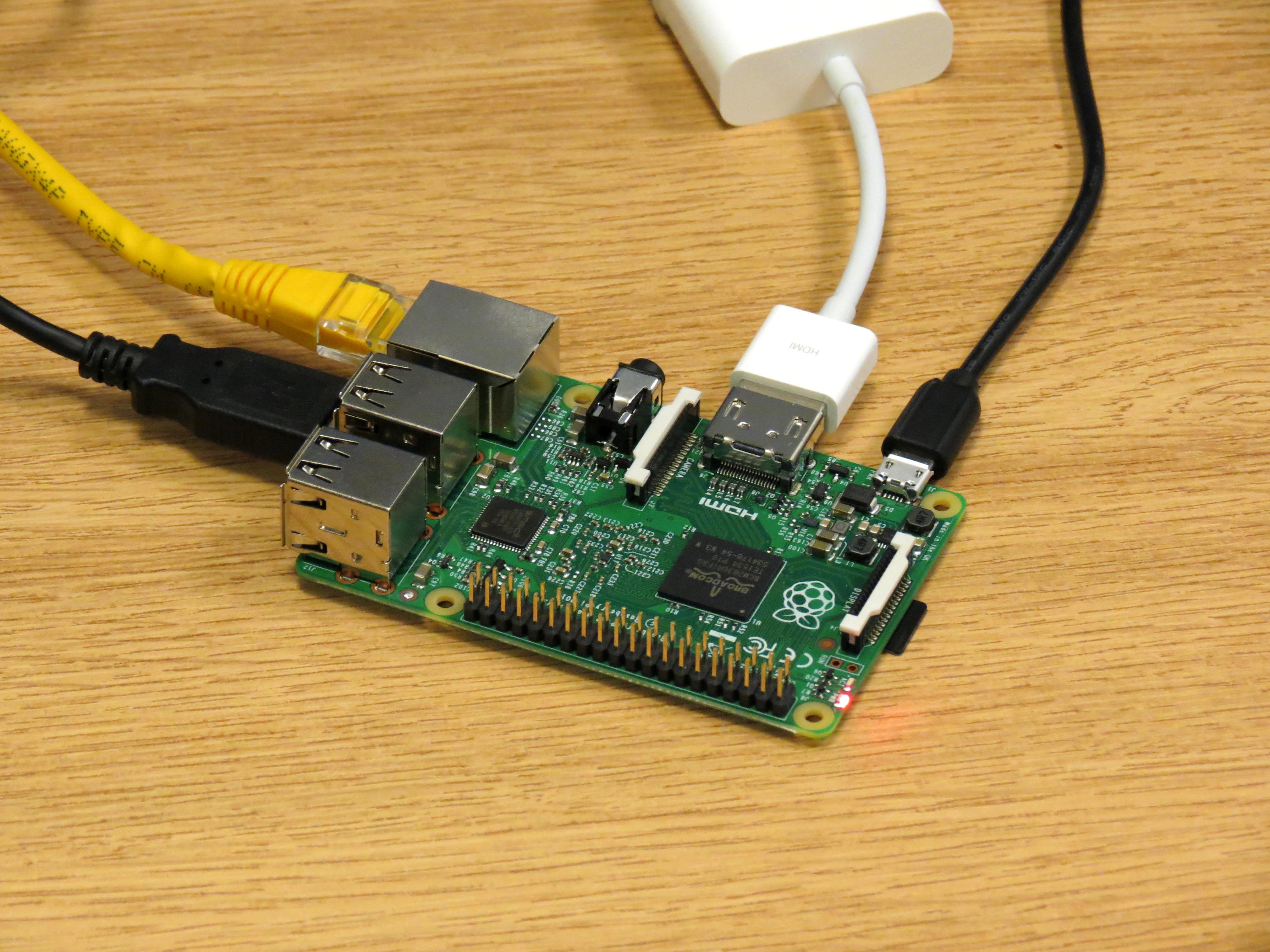
The photo at the top shows the hardware assembly used for this article. The following is required:

A Raspberry Pi 2 (Model B).
Power source (can be the USB port of another computer).
Micro SD card with at least 8 GB (below it is assumed 32 GB).
Ethernet cable and a network that provides internet access.
Optional: HDMI display and cable, USB keyboard, and possibly a USB mouse if a graphical system will be installed. Alternatively, a headless system also works, with access via SSH. Below it is assumed a display is connected.

The procedure

Step 1: Download the system image kindly prepared by Sjoerd Simons, and uncompress it:

wget https://images.collabora.co.uk/rpi2/jessie-rpi2-20150705.img.gz
gunzip jessie-rpi2-20150705.img.gz

This image contains only a minimal set of Debian Jessie packages. It uses the kernel 3.18.5, and received a few firmware and boot tweaks that are specific to the Pi 2.

Step 2: Use your favourite utility to transfer the image to the micro SD card. For example, using Linux, run the following, replacing /dev/sdX for the letter corresponding to your SD card (warning: this will erase all data stored in the card):

dd bs=1M if=jessie-rpi2-20150705.img of=/dev/sdX

In some systems, the card may be in /dev/mmcblk0 instead in /dev/sdX. If a Linux machine is not available, but instead a Mac or even Windows, the instructions to install Raspbian also apply.

Step 3: Insert the card in the Pi and boot the system. In this image, the default root password is debian (you can change it for something sensible).

Step 4: The main partition in this disk image (mounted as /) has only 2.6 GB, which is not enough. Also, often more than 1 GB of memory is needed, so swap space for virtual memory is necessary. Use fdisk (as root) to expand the main partition and to create a new partition for swap. Usually this is done interactively. If the card has exactly 32 GB, the line below can be used directly, bypassing the interactive mode. It will define a main partition with 24 GB, and the remaining, about 5 GB, will be left for swap. For cards of different sizes, run fdisk manually, or change the line below accordingly.

printf "d\n2\nn\np\n\n\n+24G\nn\np\n\n\n\nt\n3\n82\nw\n" | fdisk -uc /dev/mmcblk0

Note that, when seen from the Pi, the SD card is at /dev/mmcblk0, not /dev/sdX.

Reboot (shutdown -r now), then after logging in again, run:

resize2fs /dev/mmcblk0p2
mkswap /dev/mmcblk0p3
swapon /dev/mmcblk0p3

The swapon command enables the swap partition for immediate use. To make the change permanent for the next reboot, edit the file /etc/fstab adding:

/dev/mmcblk0p3 swap swap defaults 0 0

Step 5: Edit the /etc/apt/sources.list so as to include the official Debian packages (you can replace the server for your favourite/closer mirror):

deb http://ftp.uk.debian.org/debian/ jessie main contrib non-free

Step 6: Refresh the cached list of packages, then install FSL:

apt-get update
apt-get install fsl

Step 7: The installation is almost ready. The downloaded packages do not have the “data” directory of FSL, which contains the atlases and standard space images. To obtain these, do one of the following:

From a separate FSL installation (e.g., from a different computer), copy the contents of the ${FSLDIR}/data to the /usr/share/fsl/data of the newly installed system on the Raspberry Pi. This can be done over the network, via ssh, or after plugging in and mounting (with the correct privileges) the card in a different Linux system.
If another computer with FSL installed is not available, download FSL for CentOS or Mac (at the end of the downloads page, under “Advanced Users”), then uncompress the downloaded file, and copy the whole contents of the data directory to /usr/share/fsl/data of the Pi via ssh
If another computer is not at all accessible for this step, these files can be obtained using the Pi itself, from the command line. Logged in as root in the newly installed system, run:

cd /usr/share
wget -O- http://fsl.fmrib.ox.ac.uk/fsldownloads/fsl-5.0.9-centos6_64.tar.gz | tar xzfv - fsl/data

A last option is to skip this step, go to Step 9 below, then download and copy using a graphical web-browser from an installed desktop environment.

Step 8: Add this line to the file ~/.profile:

. /etc/fsl/fsl.sh

That’s it. All that is needed to run FSL from the command line has been done.

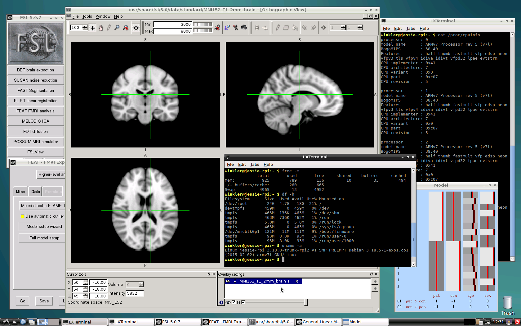
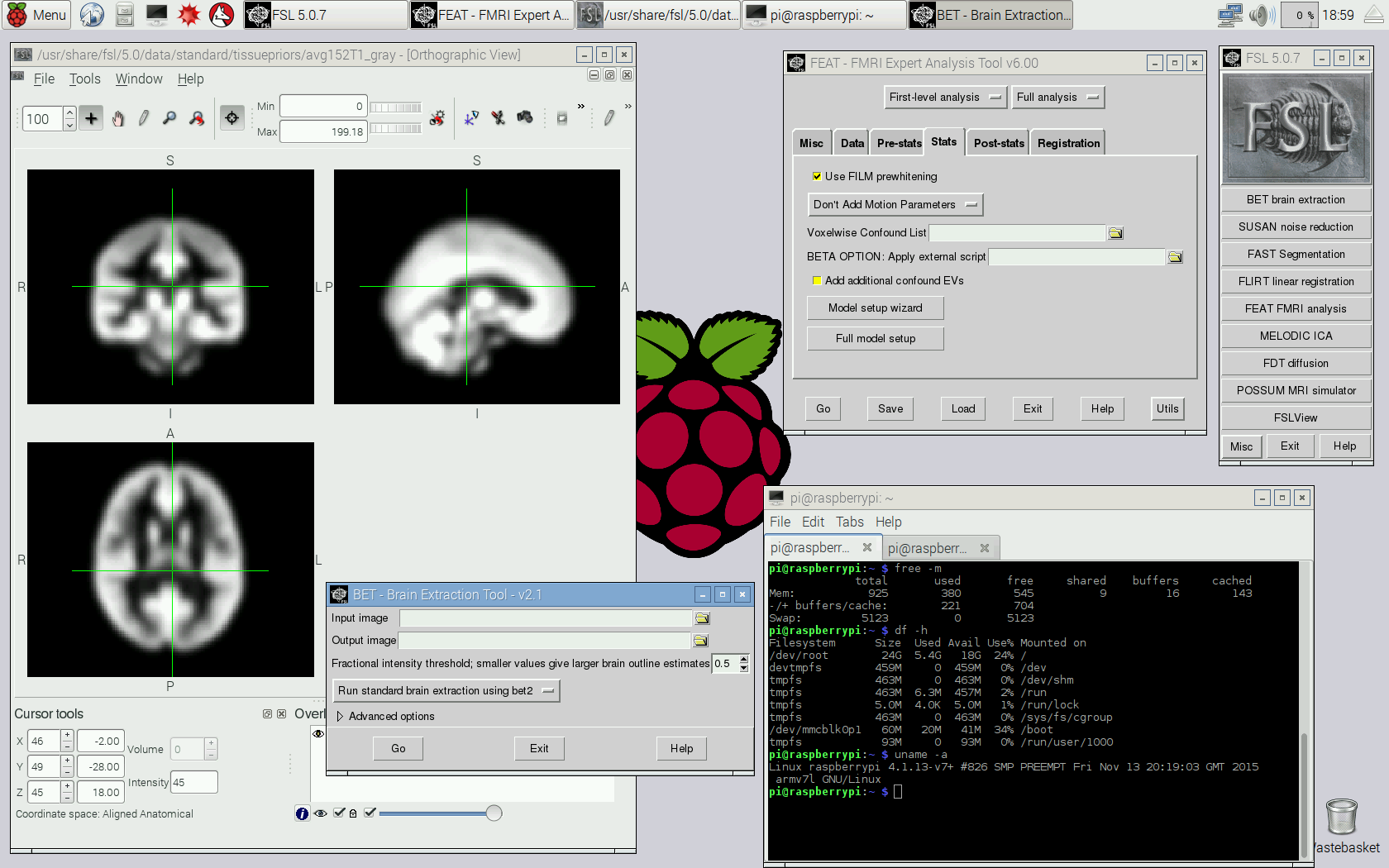
Step 9 (optional): The installation up to this step does not include a graphical user interface. To have one, install X and a desktop environment. For lightweight options, LXDE or XFCE can be considered. A screenshot of LXDE with FSLview and two terminal windows showing some system information is below (usually one would not run as root, but create an user account).

Using Raspbian

The official operating system for the Raspberry Pi, Raspbian, is a customised version of Debian, thus capable of running FSL directly. However, FSL is not in the official rpi repository. It can still be installed following similar steps as above, remembering to use sudo with commands require root privileges (the default account is rpi and the password is raspberry), and with care in the repartitioning, as the official disk image uses a different scheme. In Step 5, include the same Debian package source in the /etc/apt/sources.list file.

Overclocking

The Pi can be overclocked. Conservative, stable settings, that do not void the warranty, consist of increasing the CPU frequency to 1000 MHz (from the default 900), the GPU and SDRAM frequencies to 500 MHz (the defaults are 250 and 450 respectively), and the CPU/GPU voltage by 2 steps, i.e., by 2 × 25 mV, from 1.20 to 1.25 V. The overclock settings are adjusted in the file /boot/firmware/config.txt if using Debian (following the steps above), or in /boot/config.txt if using Raspbian:

arm_freq=1000
gpu_freq=500
sdram_freq=500
over_voltage=2

These settings cause the bogomips to jump from 38.40 to 64.00. The temperature of the onboard chips can increase, however, and a suggestion is to use heatsinks or fans, which are inexpensive and can be purchased online (fans would be powered by GPIO pins).

Performance

With the system up and running, it is time for some benchmarks. Although the assembly is exciting and in general the system speed respectable, unfortunately, processing using FEEDS suggests a poor performance. The table below compares the timings of the Pi 2 with default versus overclocked settings, relative to a minimal install of the Debian Jessie on a notebook with an Intel Core i5 processor and 8 GB of RAM.

	Default settings	Overclocked settings
PRELUDE & FUGUE	6.0	4.8
SUSAN	15.1	11.9
SIENAX	13.3	10.4
BET2	12.3	9.4
FEAT	12.1	9.6
MELODIC	15.9	12.2
FIRST	14.0	11.1
FDT	7.4	5.9
FNIRT	26.6	19.3
Total time	12.2	9.5

Running the whole FEEDS took 22 minutes in the Intel Core i5, whereas in the Pi 2 it took 4h29min with the default settings, and 3h30min after overclocking. It should be noted, however, that the 1 GB of RAM is not sufficient to run the test without using virtual memory (swapping). This needs to be taken into account when evaluating the table above. The SD card used for the tests is a Class 10, which is not as fast as actual RAM (faster cards would have their performance curtailed by hardware limits).

The performances of Debian and Raspbian on the Pi 2 are nearly identical. Running in the graphical mode (at least with LXDE) or in a console-only system do not seem to impact results, at least as far only one instance of FEEDS was running.

Conclusion

It is possible to run FSL on the Raspberry Pi 2, and the procedure is not too different than doing the same in an ordinary computer. The performance, however, suggests that the current model, being about ten times slower, may not be a competitive choice for brain imaging.

Permutation tests in the Human Connectome Project

Posted on 07.December.2015 by A. M. Winkler

Permutation tests are known to be superior to parametric tests: they are based on only few assumptions, essentially that the data are exchangeable, and allow the correction for the multiplicity of tests and the use of various non-standard statistics. The exchangeability assumption allows data to be permuted whenever their joint distribution remains unaltered. Usually this means that each observation needs to be independent from the others.

In many studies, however, there are repeated measurements on the same subjects, which violates exchangeability: clearly, the various measurements obtained from a given subject are not independent from each other. In the Human Connectome Project (HCP) (Van Essen et al, 2012; 2013; see references at the end), subjects are sampled along with their siblings (most of them are twins), such that independence cannot be guaranteed either.

In Winkler et al. (2014), certain structured types of non-independence in brain imaging were addressed through the definition of exchangeability blocks (EBs). Observations within EB can be shuffled freely or, alternatively, the EBs themselves can be shuffled as a whole. This allows various designs that otherwise could not be assessed through permutations.

The same idea can be generalised for blocks that are nested within other blocks, in a multi-level fashion. In the paper Multi-level Block Permutation (Winkler et al., 2015) we presented a method that allows blocks to be shuffled a whole, and inside them, sub-blocks are further allowed to be shuffled, in a recursive process. The method is flexible enough to accommodate permutations, sign-flippings (sometimes also called “wild bootstrap”), and permutations together with sign-flippings.

In particular, this permutation scheme allows the data of the HCP to be analysed via permutations: subjects are allowed to be shuffled with their siblings while keeping the joint distribution intra-sibship maintained. Then each sibship is allowed to be shuffled with others of the same type.

In the paper we show that the error type I is controlled at the nominal level, and the power is just marginally smaller than that would be obtained by permuting freely if free permutation were allowed. The more complex the block structure, the larger the reductions in power, although with large sample sizes, the difference is barely noticeable.

Importantly, simply ignoring family structure in designs as this causes the error rates not to be controlled, with excess false positives, and invalid results. We show in the paper examples of false positives that can arise, even after correction for multiple testing, when testing associations between cortical thickness, cortical area, and measures of body size as height, weight, and body-mass index, all of them highly heritable. Such false positives can be avoided with permutation tests that respect the family structure.

The figure at the top shows how the subjects of the HCP (terminal dots, shown in white colour) can be shuffled or not, while respecting the family structure. Blue dots indicate branches that can be permuted, whereas red dots indicate branches that cannot (see the main paper for details). This diagram includes 232 subjects of an early public release of HCP data. The tree on the left considers dizygotic twins as a category on their own, i.e., that cannot be shuffled with ordinary siblings, whereas the tree on the right considers dizygotic twins as ordinary siblings.

The first applied study using our strategy has just appeared. The method is implemented in the freely available package PALM — Permutation Analysis of Linear Models, and a set of practical steps to use it with actual HCP data is available here.

References

Van Essen DC, Ugurbil K, Auerbach E, Barch D, Behrens TE, Bucholz R, Chang A, Chen L, Corbetta M, Curtiss SW, Della Penna S, Feinberg D, Glasser MF, Harel N, Heath AC, Larson-Prior L, Marcus D, Michalareas G, Moeller S, Oostenveld R, Petersen SE, Prior F, Schlaggar BL, Smith SM, Snyder AZ, Xu J, Yacoub E; WU-Minn HCP Consortium. The Human Connectome Project: a data acquisition perspective. Neuroimage. 2012;62(4):2222-31.
Van Essen DC, Smith SM, Barch DM, Behrens TEJ, Yacoub E, Ugurbil K. The WU-Minn Human Connectome Project: An overview. Neuroimage. 2013;80:62-79.
Winkler AM, Ridgway GR, Webster MA, Smith SM, Nichols TE. Permutation inference for the general linear model. Neuroimage. 2014;92:381-97. (Open Access)
Winkler AM, Webster MA, Vidaurre D, Nichols TE, Smith SM. Multi-level block permutation. Neuroimage. 2015;123:253-68. (Open Access)

The G-statistic

Posted on 17.February.2014 by A. M. Winkler

Preliminaries

Consider the common analysis of a neuroimaging experiment. At each voxel, vertex, face or edge (or any other imaging unit), we have a linear model expressed as:

$\mathbf{Y} = \mathbf{M} \boldsymbol{\psi} + \boldsymbol{\epsilon}$

where $\mathbf{Y}$ contains the experimental data, $\mathbf{M}$ contains the regressors, $\boldsymbol{\psi}$ the regression coefficients, which are to be estimated, and $\boldsymbol{\epsilon}$ the residuals. For a linear null hypothesis $\mathcal{H}_0 : \mathbf{C}'\boldsymbol{\psi}=\mathbf{0}$ , where $\mathbf{C}$ is a contrast. If $\mathsf{rank}\left(\mathbf{C}\right) = 1$ , the Student’s t statistic can be calculated as:

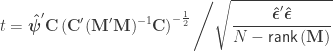
$t = \boldsymbol{\hat{\psi}}'\mathbf{C} \left(\mathbf{C}'(\mathbf{M}'\mathbf{M})^{-1}\mathbf{C} \right)^{-\frac{1}{2}} \left/ \sqrt{\dfrac{\boldsymbol{\hat{\epsilon}}'\boldsymbol{\hat{\epsilon}}}{N-\mathsf{rank}\left(\mathbf{M}\right)}} \right.$

where the hat on $\boldsymbol{\hat{\psi}}$ and $\boldsymbol{\hat{\epsilon}}$ indicate that these are quantities estimated from the sample. If $\mathsf{rank}\left(\mathbf{C}\right) \geqslant 1$ , the F statistic can be obtained as:

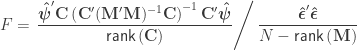
$F = \left.\dfrac{\boldsymbol{\hat{\psi}}'\mathbf{C} \left(\mathbf{C}'(\mathbf{M}'\mathbf{M})^{-1}\mathbf{C} \right)^{-1} \mathbf{C}'\boldsymbol{\hat{\psi}}}{\mathsf{rank}\left(\mathbf{C}\right)} \right/ \dfrac{\boldsymbol{\hat{\epsilon}}'\boldsymbol{\hat{\epsilon}}}{N-\mathsf{rank}\left(\mathbf{M}\right)}$

When $\mathsf{rank}\left(\mathbf{C}\right) = 1$ , $F = t^2$ . For either of these statistics, we can assess their significance by repeating the same fit after permuting $\mathbf{Y}$ or $\mathbf{M}$ (i.e., a permutation test), or by referring to the formula for the distribution of the corresponding statistic, which is available in most statistical software packages (i.e., a parametric test).

Permutation tests don’t depend on the same assumptions on which parametric tests are based. As some of these assumptions can be quite stringent in practice, permutation methods arguably should be preferred as a general framework for the statistical analysis of imaging data. At each permutation, a new statistic is computed and used to build its empirical distribution from which the p-values are obtained. In practice it’s not necessary to build the full distribution, and it suffices to increment a counter at each permutation. At the end, the counter is divided by the number of permutations to produce a p-value.

An example of a permutation distribution

Using permutation tests, correction for multiple testing using the family-wise error rate (fwer) is trivial: rather than build the permutation distribution at each voxel, a single distribution of the global maximum of the statistic across the image is constructed. Each permutation yields one maximum, that is used to build the distribution. Any dependence between the tests is implicitly captured, with not need to model it explicitly, nor to introduce even more assumptions, a problem that hinders methods such as the random field theory.

Exchangeability blocks

Permutation is allowed if it doesn’t affect the joint distribution of the error terms, i.e., if the errors are exchangeable. Some types of experiments may involve repeated measurements or other kinds of dependency, such that exchangeability cannot be guaranteed between all observations. However, various cases of structured dependency can still be accommodated if sets (blocks) of observations are shuffled as a whole, or if shuffling happens only within set (block). It is not necessary to know or to model the exact dependence structure between observations, which is captured implicitly as long as the blocks are defined correctly.

Permutation within block.

Permutation of blocks as a whole.

The two figures above are of designs constructed using the fsl software package. In fsl, within-block permutation is available in randomise with the option -e, used to supply a file with the definition of blocks. For whole-block permutation, in addition to the option -e, the option --permuteBlocks needs to be supplied.

The G-statistic

The presence of exchangeability blocks solves a problem, but creates another. Having blocks implies that observations may not be pooled together to produce a non-linear parameter estimate such as the variance. In other words: the mere presence of exchangeability blocks, either for shuffling within or as a whole, implies that the variances may not be the same across all observations, and a single estimate of this variance is likely to be inaccurate whenever the variances truly differ, or if the groups don’t have the same size. This also means that the F or t statistics may not behave as expected.

The solution is to use the block definitions and the permutation strategy is to define groups of observations that are known or assumed to have identical variances, and pool only the observations within group for variance estimation, i.e., to define variance groups (vgs).

The F-statistic, however, doesn’t allow such multiple groups of variances, and we need to resort to another statistic. In Winkler et al. (2014) we propose:

$G = \dfrac{\boldsymbol{\hat{\psi}}'\mathbf{C} \left(\mathbf{C}'(\mathbf{M}'\mathbf{W}\mathbf{M})^{-1}\mathbf{C} \right)^{-1} \mathbf{C}'\boldsymbol{\hat{\psi}}}{\Lambda \cdot s}$

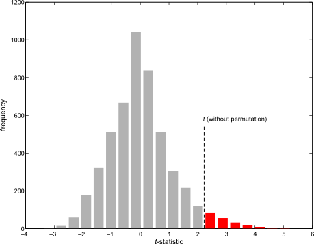
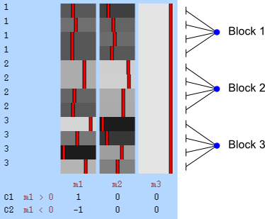
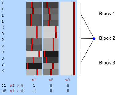
where $\mathbf{W}$ is a diagonal matrix that has elements:

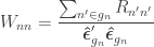
$W_{nn}=\dfrac{\sum_{n' \in g_{n}}R_{n'n'}}{\boldsymbol{\hat{\epsilon}}_{g_{n}}'\boldsymbol{\hat{\epsilon}}_{g_{n}}}$

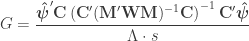
and where $R_{n'n'}$ are the $n'$ diagonal elements of the residual forming matrix, and $g_{n}$ is the variance group to which the $n$ -th observation belongs. The remaining denominator term, $\Lambda$ , is given by (Welch, 1951):

$\Lambda = 1+\frac{2(s-1)}{s(s+2)}\sum_{g} \frac{1}{\sum_{n \in g}R_{nn}} \left(1-\frac{\sum_{n \in g}W_{nn}}{\mathsf{trace}\left(\mathbf{W}\right)}\right)^2$

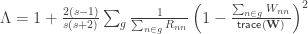
where $s=\mathsf{rank}\left(\mathbf{C}\right)$ . The matrix $\mathbf{W}$ can be seen as a weighting matrix, the square root of which normalises the model such that the errors have then unit variance and can be ignored. It can also be seen as being itself a variance estimator. In fact, it is the very same variance estimator proposed by Horn et al (1975).

The W matrix used with the G statistic. It is constructed from the estimated variances of the error terms.

The matrix $\mathbf{W}$ has a crucial role in making the statistic pivotal in the presence of heteroscedasticity. Pivotality means that the statistic has a sampling distribution that is not dependent on any unknown parameter. For imaging experiments, it’s important that the statistic has this property, otherwise correction for multiple testing that controls fwer will be inaccurate, or possibly invalid altogether.

When $\mathsf{rank}\left(\mathbf{C}\right)=1$ , the t-equivalent to the G-statistic is 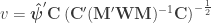$v = \boldsymbol{\hat{\psi}}'\mathbf{C} \left(\mathbf{C}'(\mathbf{M}'\mathbf{W}\mathbf{M})^{-1}\mathbf{C} \right)^{-\frac{1}{2}}$ , which is the well known Aspin-Welch $v$ -statistic for the Behrens-Fisher problem. The relationship between $v$ and G is the same as between t and F, i.e., when the rank of the contrast equals to one, the latter is simply the square of the former. The G statistic is a generalization of all these, and more, as we show in the paper, and summarise in the table below:

	$\mathsf{rank}\left(\mathbf{C}\right) = 1$	$\mathsf{rank}\left(\mathbf{C}\right) > 1$
Homoscedastic errors, unrestricted exchangeability	Square of Student’s t	F-ratio
Homoscedastic within vg, restricted exchangeability	Square of Aspin-Welch $v$	Welch’s $v^2$

In the absence of variance groups (i.e., all observations belong to the same vg), G and $v$ are equivalent to F and t respectively.

Although not typically necessary if permutation methods are to be preferred, approximate parametric p-values for the G-statistic can be computed from an F-distribution with $\nu_1=s$ and $\nu_2=2(s-1)/3/(\Lambda-1)$ .

While the error rates are controlled adequately (a feature of permutation tests in general), the G-statistic offers excellent power when compared to the F-statistic, even when the assumptions of the latter are perfectly met. Moreover, by preserving pivotality, it is an adequate statistic to control of the error rate in the in the presence of multiple tests.

In this post, the focus is in using G for imaging data, but of course, it can be used for any dataset in which a linear model where variances cannot be assumed to be the same is used, i.e., when heteroscedasticity is or could be present.

Note that the G-statistic has nothing to do with the G-test. It is named as this for being a generalisation over various tests, including the commonly used t and F tests, as shown above.

Main reference

The core reference and results for the G-statistic have just been published in Neuroimage:

Winkler AM, Ridgway GR, Webster MA, Smith SM, Nichols TE. Permutation inference for the general linear model. Neuroimage. 2014;92:381-397

Other references

The two other references cited, which are useful to understand the variance estimator and the parametric approximation are:

Horn S, Horn R, Duncan D. Estimating heteroscedastic variances in linear models. J Am Stat Assoc. 1975;70(350):380–385.
Welch B. On the comparison of several mean values: an alternative approach. Biometrika. 1951;38(3):330–336.

Automatic atlas queries in FSL

Posted on 30.July.2012 by A. M. Winkler

The fmrib Software Library (fsl) provides a tool to query whether regions belong or not to one of various atlases available. This well-known tool is called atlasquery, and it requires one region per image per run. To run for multiple separate regions on a single image image (e.g., a thresholded statistical map), a separate call to fsl‘s cluster command (not to be confused with the homonym cluster command that is part of the GraphViz package) is needed.

In order to automate this task, a small script called autoaq is available (UPDATE: the script is no longer supplied here; it has been incorporated into fsl). Usage information is provided by calling the command without arguments. This is the same script we posted recently to the fsl mailing list (here). Obviously, it does not run in Microsoft Windows. To use it, you need any recent Linux or Mac computer with fsl installed.

An example call is shown below:

./autoaq -i pvals.nii.gz -t 0.95 -o report.txt -a "JHU White-Matter Tractography Atlas"

The command will write temporary files to the directory from where it is called, hence it needs to be called from a directory to which the user has writing permissions. The atlas name can be any of the atlases available in fsl, currently being the ones listed below (note the quotes, ” “, that need to be provided when calling autoaq):

“Cerebellar Atlas in MNI152 space after normalization with FLIRT”
“Cerebellar Atlas in MNI152 space after normalization with FNIRT”
“Harvard-Oxford Cortical Structural Atlas”
“Harvard-Oxford Subcortical Structural Atlas”
“JHU ICBM-DTI-81 White-Matter Labels”
“JHU White-Matter Tractography Atlas”
“Juelich Histological Atlas”
“MNI Structural Atlas”
“Oxford Thalamic Connectivity Probability Atlas”
“Oxford-Imanova Striatal Connectivity Atlas 3 sub-regions”
“Oxford-Imanova Striatal Connectivity Atlas 7 sub-regions”
“Oxford-Imanova Striatal Structural Atlas”
“Talairach Daemon Labels”

The list can always be obtained through atlasquery --dumpatlases. Information about these atlases is available here.

The output is divided in three sections. In the first, a table containing the cluster indices, size and coordinates of the peaks and centres of mass is provided. In the second part, the structures to which the cluster peaks belong are presented, along with the associated probabilities. In the third part, probabilities for each cluster as a whole is presented. If the atlas is a binary label atlas, the number shown is in fact the overlap percentage between the cluster and the respective atlas label. If the atlas is probabilistic, the value is the mean probability in the overlapping region.

Version history:

03.Oct.2012: Update – Fixed issue with the md5 command under a different name in vanilla Mac.
25.Jan.2014: Update – Added options -u (to update/append a previous report) and -p to show peak coordinates instead of center of mass.
10.Dec.2014: The autoaq has been integrated into the freely available fmrib Software Library (fsl) and is no longer provided here. Hope you enjoy using it directly into fsl! :-)