multivariate | Brainder.

In canonical correlation analysis (CCA; Hotelling, 1936), the absolute value of a correlation is not always that helpful. For example, large canonical correlations may arise simply due to a large number of variables being investigated using a relatively small sample size; high correlations may arise simply because there are too many opportunities for finding mixtures in both sides that are highly correlated one with another.

Motivated by this perceived difficulty in the interpretation of results, Stewart and Love (1968) proposed the computation of what has been termed a redundancy index. It works as follows.

Let $\mathbf{Y}_{N \times P}$ and $\mathbf{X}_{N \times Q}$ be two sets of variables over which CCA is computed. We find canonical coefficients $\mathbf{A}_{P \times K}$ and $\mathbf{B}_{Q \times K}$ , $K=\min(P,Q)$ such that the canonical variables $\mathbf{U}_{N \times K}$ and $\mathbf{V}_{N \times K}$ have maximal, diagonal correlation structure; this diagonal contains the ordered canonical correlations $r_k$ .

Now that CCA has been computed, we can find the correlations between the original variables and the canonical coefficients. Let $\mathbf{\tilde{A}}_{P \times K}=\text{corr}(\mathbf{Y},\mathbf{U})$ and $\mathbf{\tilde{B}}_{Q \times K}=\text{corr}(\mathbf{X},\mathbf{V})$ be such correlations, which are termed canonical loadings or structure coefficients. Now compute the mean square for each of the columns of $\mathbf{\tilde{A}}$ and $\mathbf{\tilde{B}}$ . These represent the variance extracted by the corresponding canonical variable. That is:

Variance extracted by canonical variable $\mathbf{u}_{k}$ : $\upsilon_k = \frac{1}{P}\sum_{p=1}^{P}\tilde{a}_{pk}^{2}$
Variance extracted by canonical variable $\mathbf{v}_{k}$ : $\nu_k = \frac{1}{Q}\sum_{q=1}^{Q}\tilde{b}_{qk}^{2}$

These quantities represent the mean variance extracted from the original variables by each of the canonical variables (in each side).

Compute now the proportion of variance of one canonical variable (say, $\mathbf{u}_{k}$ ) explained by the corresponding canonical variable in the other side (say, $\mathbf{v}_{k}$ ). This is given simply by $r_k^2$ , the usual coefficient of determination.

The redundancy index for each canonical variable is then the product of $\upsilon_k$ and $r_k^2$ for the left side of CCA, and the product of $\nu_k$ and $r_k^2$ for the right side. That is, the index is not symmetric. It measures the proportion of variance in one of the two set of variables explained by the correlation between the $k$ -th pair of canonical variables.

The sum of the redundancies for all $K$ canonical variables in one side or another forms a global redundancy metric, which indicates the proportion of the variance in a given side explained by the variance in the other.

This global redundancy can be scaled to unity, such that the redundancies for each of the canonical variables in a give side can be interpreted as the proportion of total redundancy.

If you follow the original paper by Stewart and Love (1968), $\upsilon_k$ and $\nu_k$ are column III of Table 2, the redundancy of each canonical variable for each side corresponds to column IV, and the proportion of total redundancy is in column V.

Another reference on the same topic that is worth looking is Miller (1981). In it, the author discusses that redundancy is somewhere in between CCA itself (fully symmetric) and multiple regression (fully asymmetric).

Reference

Hotelling H. Relations between two sets of variates. Biometrika. 1936;28(3/4):321–77.
Muller KE. Relationships between redundancy analysis, canonical correlation, and multivariate regression. Psychometrika. 1981;46(2):139–42.
Stewart D, Love W. A general canonical correlation index. Psychological Bulletin. 1968;70(3, Pt.1):160–3. (unfortunately, the paper is paywalled; write to APA to complain).

Update

28.Jun.2020: A script that computes the redundancy indices is available here: redundancy.m (work with Thomas Wassenaar, University of Oxford).

It’s so often that we find ourselves in the need to quickly compute a statistic for a certain dataset, but finding the formulas is not always direct. Using a statistical software is helpful, but it often also happens that the reported results are not exactly what one may believe it represents. Moreover, even if using these packages, it is always good to have in mind the meaning of statistics and how they are computed. Here the formulas for the most commonly used statistics with the general linear model (glm) are presented, all in matrix form, that can be easily implemented in Octave or Matlab.

I — Model

We consider two models, one univariate, another multivariate. The univariate is a particular case of the multivariate, but for univariate problems, it is simpler to use the smaller, particular case.

Univariate model

The univariate glm can be written as:

$\mathbf{y} = \mathbf{M}\boldsymbol{\psi} + \boldsymbol{\epsilon}$

where $\mathbf{y}$ is the $N \times 1$ vector of observations, $\mathbf{M}$ is the $N \times s$ matrix of explanatory variables, $\boldsymbol{\psi}$ is the $s \times 1$ vector of regression coefficients, and $\boldsymbol{\epsilon}$ is the $N \times 1$ vector of residuals.

The null hypothesis can be stated as $\mathcal{H}_0 : \mathbf{C}'\boldsymbol{\psi} = 0$ , where $\mathbf{C}$ is a $s \times s'$ matrix that defines a contrast of regression coefficients, satisfying $\mathsf{rank}(\mathbf{C}) = s'$ and $1 \geqslant s' \geqslant s$ .

Multivariate model

The multivariate glm can be written as:

$\mathbf{Y} = \mathbf{M}\boldsymbol{\Psi} + \boldsymbol{\epsilon}$

where $\mathbf{Y}$ is the $N \times q$ vector of observations, $\mathbf{M}$ is the $N \times s$ matrix of explanatory variables, $\boldsymbol{\Psi}$ is the $s \times q$ vector of regression coefficients, and $\boldsymbol{\epsilon}$ is the $N \times q$ vector of residuals.

The null hypothesis can be stated as $\mathcal{H}_0 : \mathbf{C}'\boldsymbol{\Psi}\mathbf{D} = 0$ , where $\mathbf{C}$ is defined as above, and $\mathbf{D}$ is a $q \times q'$ matrix that defines a contrast of observed variables, satisfying $\mathsf{rank}(\mathbf{D}) = q'$ and $1 \geqslant q' \geqslant q$ .

II — Estimation of parameters

In the model, the unknowns of interest are the values arranged in $\boldsymbol{\Psi}$ . These can be estimated as:

$\boldsymbol{\hat{\Psi}} = (\mathbf{M}'\mathbf{M})^{+}(\mathbf{M}'\mathbf{Y})$

where the $^{+}$ represents a pseudo-inverse. The residuals can be computed as:

$\boldsymbol{\hat{\epsilon}} = \mathbf{Y} - \mathbf{M}\boldsymbol{\hat{\Psi}}$

The above also applies to the univariate case ( $\mathbf{y}$ is a particular case of $\mathbf{Y}$ , and $\boldsymbol{\psi}$ of $\boldsymbol{\Psi}$ ).

III – Univariate statistics

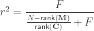
Coefficient of determination, R²

The following is the fraction of the variance explained by the part of the model determined by the contrast. It applies to mean-centered data and design, i.e., $\tilde{\mathbf{y}}=\mathbf{y}-\bar{y}$ and $\tilde{\mathbf{M}}=\mathbf{M}-\bar{\mathbf{m}}$ .

$R^2 = \dfrac{\boldsymbol{\hat{\psi}}'\mathbf{C} \left(\mathbf{C}'(\tilde{\mathbf{M}}'\tilde{\mathbf{M}})^{-1}\mathbf{C} \right)^{-1} \mathbf{C}'\boldsymbol{\hat{\psi}}}{\tilde{\mathbf{y}}'\tilde{\mathbf{y}}}$

Note that the portion of the variance explained by nuisance variables (if any) remains in the denominator. To have these taken into account, consider the squared partial correlation coefficient, or Pillai’s trace with univariate data, both described further down.

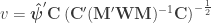
Pearson’s correlation coefficient

When $\mathsf{rank}\left(\mathbf{C}\right) = 1$ , the multiple correlation coefficient can be computed from the $R^2$ statistic as:

$R = \mathsf{sign}\left(\mathbf{C}'\boldsymbol{\hat{\psi}}\right)\sqrt{R^2}$

This value should not be confused, even in the presence of nuisance, with the partial correlation coefficient (see below).

Student’s t statistic

If $\mathsf{rank}\left(\mathbf{C}\right) = 1$ , the Student’s $t$ statistic can be computed as:

$t = \boldsymbol{\hat{\psi}}'\mathbf{C} \left(\mathbf{C}'(\mathbf{M}'\mathbf{M})^{-1}\mathbf{C} \right)^{-\frac{1}{2}} \left/ \sqrt{\dfrac{\boldsymbol{\hat{\epsilon}}'\boldsymbol{\hat{\epsilon}}}{N-\mathsf{rank}\left(\mathbf{M}\right)}} \right.$

F statistic

The $F$ statistic can be computed as:

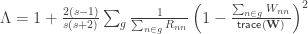
$F = \left.\dfrac{\boldsymbol{\hat{\psi}}'\mathbf{C} \left( \mathbf{C}'(\mathbf{M}'\mathbf{M})^{-1}\mathbf{C} \right)^{-1} \mathbf{C}'\boldsymbol{\hat{\psi}}}{\mathsf{rank}\left(\mathbf{C} \right)} \right/ \dfrac{\boldsymbol{\hat{\epsilon}}'\boldsymbol{\hat{\epsilon}}}{N-\mathsf{rank}\left(\mathbf{M}\right)}$

Aspin—Welch v

If homoscedastic variances cannot be assumed, and $\mathsf{rank}\left(\mathbf{C}\right) = 1$ , this is equivalent to the Behrens—Fisher problem, and the Aspin—Welch’s $t$ statistic can be computed as:

$v = \boldsymbol{\hat{\psi}}'\mathbf{C} \left(\mathbf{C}'(\mathbf{M}'\mathbf{W}\mathbf{M})^{-1}\mathbf{C} \right)^{-\frac{1}{2}}$

where $\mathbf{W}$ is a diagonal matrix that has elements:

$W_{nn}=\dfrac{\sum_{n' \in g_{n}}R_{n'n'}}{\boldsymbol{\hat{\epsilon}}_{g_{n}}'\boldsymbol{\hat{\epsilon}}_{g_{n}}}$

and where $R_{n'n'}$ are the $n'$ diagonal elements of the residual forming matrix $\mathbf{R} = \mathbf{I}-\mathbf{M}\mathbf{M}^{+}$ , and $g_{n}$ is the variance group to which the $n$ -th observation belongs.

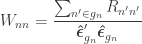
Generalised G statistic

If variances cannot be assumed to be the same across all observations, a generalisation of the $F$ statistic can be computed as:

$G = \dfrac{\boldsymbol{\hat{\psi}}'\mathbf{C} \left(\mathbf{C}'(\mathbf{M}'\mathbf{W}\mathbf{M})^{-1}\mathbf{C} \right)^{-1} \mathbf{C}'\boldsymbol{\hat{\psi}}}{\Lambda \cdot \mathsf{rank}\left(\mathbf{C}\right)}$

where $\mathbf{W}$ is defined as above, and the remaining denominator term, $\Lambda$ , is given by:

$\Lambda = 1+\frac{2(s-1)}{s(s+2)}\sum_{g} \frac{1}{\sum_{n \in g}R_{nn}} \left(1-\frac{\sum_{n \in g}W_{nn}}{\mathsf{trace}\left(\mathbf{W}\right)}\right)^2$

There is another post on the G-statistic (here).

Partial correlation coefficient

When $\mathsf{rank}\left(\mathbf{C}\right) = 1$ , the partial correlation can be computed from the Student’s $t$ statistic as:

$r = \mathsf{sign}\left(t\right)\sqrt{\dfrac{t^2}{N-\mathsf{rank}\left(\mathbf{M}\right)+t^2}}$

The square of the partial correlation corresponds to Pillai’s trace applied to an univariate model, and it can also be computed from the $F$ -statistic as:

$r^2 = \dfrac{F}{\frac{N-\mathsf{rank}\left(\mathbf{M}\right)}{\mathsf{rank}\left(\mathbf{C}\right)}+F}$

Likewise, if $r$ is known, the formula can be solved for $t$ :

$t = \dfrac{r\sqrt{N-\mathsf{rank}\left(\mathbf{M}\right)}}{\sqrt{1-r^2}}$

or for $F$ :

$F = \dfrac{r^2}{1-r^2}\times\dfrac{N-\mathsf{rank}\left(\mathbf{M}\right)}{\mathsf{rank}\left(\mathbf{C}\right)}$

The partial correlation can also be computed at once for all variables vs. all other variables as follows. Let $\mathbf{A} = \left[\mathbf{y}\; \mathbf{M}\right]$ , and $\mathsf{r}\left(\mathbf{A}\right)$ be the inverse of the correlation matrix of the columns of $\mathbf{A}$ , and $\mathsf{d}\left(\cdot\right)$ the diagonal operator, that returns a column vector with the diagonal entries of a square matrix. Then the matrix with the partial correlations is:

$\mathbf{r} = -\mathsf{r}\left(\mathbf{A}\right) \odot \left(\mathsf{d}\left(\mathsf{r}\left(\mathbf{A}\right)\right)\mathsf{d}\left(\mathsf{r}\left(\mathbf{A}\right)\right)'\right)^{-\frac{1}{2}}$

where $\odot$ is the Hadamard product, and the power “ $-\frac{1}{2}$ ” is taken elementwise (i.e., not matrix power).

IV – Multivariate statistics

For the multivariate statistics, define generically $\mathbf{E} = (\boldsymbol{\hat{\epsilon}}\mathbf{D})'(\boldsymbol{\hat{\epsilon}}\mathbf{D})$ as the sums of the products of the residuals, and $\mathbf{H}=(\mathbf{C}'\boldsymbol{\hat{\Psi}}\mathbf{D})' \left(\mathbf{C}'(\mathbf{M}'\mathbf{M})^{-1}\mathbf{C} \right)^{-1} (\mathbf{C}'\boldsymbol{\hat{\Psi}}\mathbf{D})$ as the sums of products of the hypothesis. In fact, the original model can be modified as $\tilde{\mathbf{Y}} = \mathbf{M}\tilde{\boldsymbol{\Psi}} + \tilde{\boldsymbol{\epsilon}}$ , where $\tilde{\mathbf{Y}}=\mathbf{Y}\mathbf{D}$ , $\tilde{\boldsymbol{\Psi}} = \boldsymbol{\Psi}\mathbf{D}$ and $\tilde{\boldsymbol{\epsilon}}=\boldsymbol{\epsilon}\mathbf{D}$ .

If $\mathsf{rank}\left(\mathbf{D}\right)=1$ , this is an univariate model, otherwise it remains multivariate, although $\mathbf{D}$ can be omitted from the formulas. From now on this simplification is adopted, so that $\mathbf{E} = \boldsymbol{\hat{\epsilon}}'\boldsymbol{\hat{\epsilon}}$ and $\mathbf{H}=\boldsymbol{\hat{\Psi}}'\mathbf{C} \left(\mathbf{C}'(\mathbf{M}'\mathbf{M})^{-1}\mathbf{C} \right)^{-1} \mathbf{C}'\boldsymbol{\hat{\Psi}}$ .

Hotelling T²

If $\mathsf{rank}\left(\mathbf{C}\right) = 1$ , the Hotelling’s $T^2$ statistic can be computed as:

$T^2 = \mathbf{C}'\boldsymbol{\hat{\Psi}}\boldsymbol{\Sigma}^{-\frac{1}{2}}\left(\mathbf{C}'(\mathbf{M}'\mathbf{M})^{-1}\mathbf{C} \right)^{-1}\boldsymbol{\Sigma}^{-\frac{1}{2}} \boldsymbol{\hat{\Psi}}'\mathbf{C}$

where $\boldsymbol{\Sigma} = \mathbf{E}/\left(N-\mathsf{rank}\left(\mathbf{M}\right)\right)$

Multivariate alternatives to the F statistic

Classical manova/mancova statistics can be based in the ratio between the sums of products of the hypothesis and the sums of products of the residuals, or the ratio between the sums of products of the hypothesis and the total sums of products. In other words, define:

$\begin{array}{ccl} \mathbf{A} &=& \mathbf{H}\mathbf{E}^{-1} = \mathbf{E}^{-\frac{1}{2}} \boldsymbol{\hat{\psi}}'\mathbf{C} \left(\mathbf{C}'(\mathbf{M}'\mathbf{M})^{-1}\mathbf{C} \right)^{-1} \mathbf{C}'\boldsymbol{\hat{\psi}}\mathbf{E}^{-\frac{1}{2}}\\ \mathbf{B} &=& \mathbf{H}\left(\mathbf{E}+\mathbf{H}\right)^{-1} \end{array}$

Let $\lambda_i$ be the eigenvalues of $\mathbf{A}$ , and $\theta_i$ the eigenvalues of $\mathbf{B}$ . Then:

Wilks’ $\Lambda = \prod_{i} \dfrac{1}{1+\lambda_i} = \dfrac{|\mathbf{E}|}{|\mathbf{E}+\mathbf{H}|}$ .
Lawley–Hotelling’s trace: $\sum_i \lambda_i = \mathsf{trace}\left(\mathbf{A}\right)$ .
Pillai’s trace: $\sum_i \dfrac{\lambda_i}{1+\lambda_i} = \sum_i \theta_i = \mathsf{trace}\left(\mathbf{B}\right)$ .
Roy’s largest root (ii): $\lambda_1 = \mathsf{max}_i\left(\lambda_i\right) = \dfrac{\theta_1}{1-\theta_1}$ (analogous to $F$ ).
Roy’s largest root (iii): $\theta_1 = \mathsf{max}_i\left(\theta_i\right) = \dfrac{\lambda_1}{1+\lambda_1}$ (analogous to $R^2$ ).

When $\mathsf{rank}\left(\mathbf{C}\right) = 1$ , or when $\mathbf{Y}$ is univariate, or both, Lawley–Hotelling’s trace is equal to Roy’s (ii) largest root, Pillai’s trace is equal to Roy’s (iii) largest root, and Wilks’ $\Lambda$ added to Pillai’s trace equals to unity. The value $\rho_i=\sqrt{\theta_i}$ is the $i$ -th canonical correlation.