
In canonical correlation analysis (CCA; Hotelling, 1936), the absolute value of a correlation is not always that helpful. For example, large canonical correlations may arise simply due to a large number of variables being investigated using a relatively small sample size; high correlations may arise simply because there are too many opportunities for finding mixtures in both sides that are highly correlated one with another.
Motivated by this perceived difficulty in the interpretation of results, Stewart and Love (1968) proposed the computation of what has been termed a redundancy index. It works as follows.
Let 


Now that CCA has been computed, we can find the correlations between the original variables and the canonical coefficients. Let 


- Variance extracted by canonical variable
:
- Variance extracted by canonical variable
:

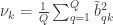
These quantities represent the mean variance extracted from the original variables by each of the canonical variables (in each side).
Compute now the proportion of variance of one canonical variable (say, 
The redundancy index for each canonical variable is then the product of 


The sum of the redundancies for all 
This global redundancy can be scaled to unity, such that the redundancies for each of the canonical variables in a give side can be interpreted as the proportion of total redundancy.
If you follow the original paper by Stewart and Love (1968),
Another reference on the same topic that is worth looking is Miller (1981). In it, the author discusses that redundancy is somewhere in between CCA itself (fully symmetric) and multiple regression (fully asymmetric).
Reference
- Hotelling H. Relations between two sets of variates. Biometrika. 1936;28(3/4):321–77.
- Muller KE. Relationships between redundancy analysis, canonical correlation, and multivariate regression. Psychometrika. 1981;46(2):139–42.
- Stewart D, Love W. A general canonical correlation index. Psychological Bulletin. 1968;70(3, Pt.1):160–3. (unfortunately, the paper is paywalled; write to APA to complain).
Update
- 28.Jun.2020: A script that computes the redundancy indices is available here: redundancy.m (work with Thomas Wassenaar, University of Oxford).
