Coefficients to assess the genetic resemblance between individuals were presented in the last post. Among these, the coefficient of kinship, , is probably the most interesting. It gives a probabilistic estimate that a random gene from a given subject is identical by descent (ibd) to a gene in the same locus from a subject . For subjects, these probabilities can be assembled in a matrix termed kinship matrix, usually represented as , that has elements , and that can be used to model the covariance between individuals in quantitative genetics.

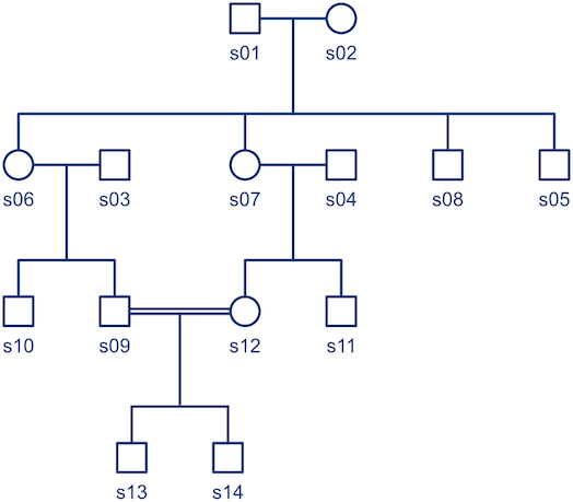
Consider the pedigree in the figure below, consisted of 14 subjects:

The corresponding kinship matrix, already multiplied by two to indicate expected covariances between subjects (i.e., ), is:

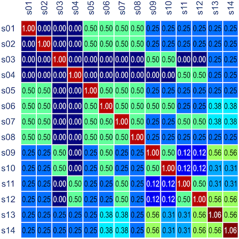
Note that the diagonal elements can have values above unity, given the consanguineous mating in the family (between s09 and s12, indicated by the double line in the pedigree diagram).

In the next post, details on how the kinship matrix can be used investigate heritabilities, genetic correlations, and to perform association studies will be presented.