July | 2013 | Brainder.

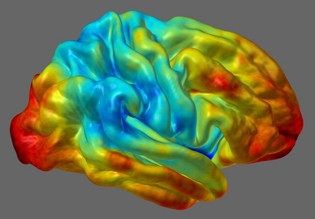
In a previous post, a method to display FreeSurfer cortical regions in arbitrary colours was presented. Suppose that, instead, you would like to display the results from vertexwise or facewise analyses. For vertexwise, these can be shown using tksurfer or Freeview. The same does not apply, however, to facewise data, which, at the time of this writing, is not available in any neuroimaging software. In this article a tool to generate files with facewise or vertexwise data is provided, along with some simple examples.

The dpx2map tool

The tool to generate the maps is dpx2map (right-click to download, then make it executable). Call it without arguments to get usage information. This tool uses Octave as the backend, and it assumes that it is installed in its usual location (/usr/bin/octave). It is also possible to run it from inside Octave or Matlab using a slight variant, dpx2map.m (in which case, type help dpx2map for usage).

In either case, the commands srfread, dpxread and mtlwrite must be available. These are part of the areal package discussed here. And yes, dpx2map is now included in the latest release of the package too.

To use dpx2map, you need to specify a surface object that will provide the geometry on which the data colours will be overlaid, and the data itself. The surface should be in FreeSurfer format (*.asc or *.srf), and the data should be in FreeSurfer “curvature” format (*.asc, *.dpv) for vertexwise, or in facewise format (*.dpf). A description of these formats is available here.

It is possible to specify the data range that will be used when computing the scaling to make the colours, as well which range will be actually shown. It is also possible to split the scale so that a central part of it is omitted or shown in a colour outside the colourscale. This is useful to show thresholded positive and negative maps.

The output is saved either in Stanford Polygon (*.ply) for vertexwise, or in Wavefront Object (*.obj + *.mtl) for facewise data, and can be imported directly in many computer graphics software. All input and output files must be/are in their respective ascii versions, not binary. The command also outputs a image with the colourbar, in Portable Network Graphics format (*.png).

An example object

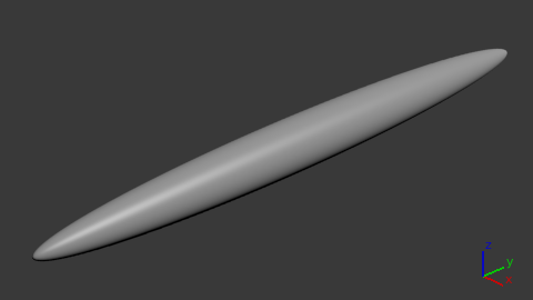
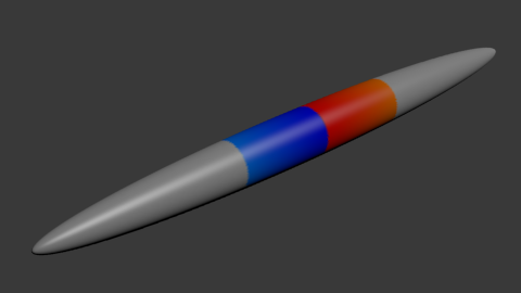
With a simple geometric shape as this it is much simpler to demonstrate how to generate the maps, than using a complicated object as the brain. The strategy for colouring remains the same. For the next examples, an ellipsoid was created using the platonic command. The command line used was:

platonic ellipsoid.obj ico sph 7 '[.25 0 0 0; 0 3 0 0; 0 0 .25 0; 0 0 0 1]'

This ellipsoid has maximum y-coordinate equal to 3, and a maximum x- and z-coordinates equal to 0.25. This file was converted from Wavefront *.obj to FreeSurfer ascii, and scalar fields simply describing the coordinates (x,y,z), were created with:

obj2srf ellipsoid.obj > ellipsoid.srf
srf2area ellipsoid.srf ellipsoid.dpv dpv
gawk '{print $1,$2,$3,$4,$2}' ellipsoid.dpv > ellipsoid-x.dpv
gawk '{print $1,$2,$3,$4,$3}' ellipsoid.dpv > ellipsoid-y.dpv
gawk '{print $1,$2,$3,$4,$4}' ellipsoid.dpv > ellipsoid-z.dpv

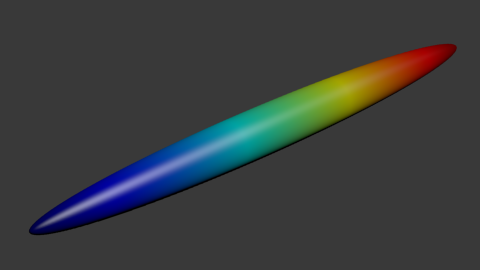
It is the ellipsoid-y.dpv that is used for the next examples.

Vertexwise examples

The examples below use the same surface (*.srf) and the same curvature, data-per-vertex file (*.dpv). The only differences are the way as the map is generated and presented, using different colour maps and different scaling. The jet colour map is the same available in Octave and Matlab. The coolhot5 is a custom colour map that will be made available, along with a few others, in another article to be posted soon.

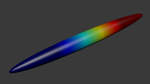
Example A

In this example, defaults are used. The input files are specified, along with a prefix (exA) to be used to name the output files.

dpx2map ellipsoid-y.dpv ellipsoid.srf exA

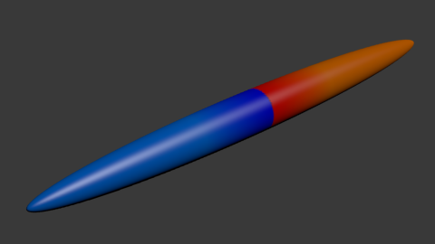
Example B

In this example, the data between values -1.5 and 1.5 is coloured, and the remaining receive the colours of the extreme points (dark blue and dark red).

dpx2map ellipsoid-y.dpv ellipsoid.srf exB jet '[-1.5 1.5]'

Example C

In this example, the data between -2 and 2 is used to define the colours, with the values below/above receiving the extreme colours. However, the range between -1 and 1 is not shown or used for the colour scaling. This is because the dual option is set as true as well as the coption.

dpx2map ellipsoid-y.dpv ellipsoid.srf exC coolhot5 '[-2 2]' '[-1 1]' true '[.75 .75 .75]' true

Example D

This example is similar as above, except that the values between -1 and 1, despite not being shown, are used for the scaling of the colours. This is due to the coption being set as true.

dpx2map ellipsoid-y.dpv ellipsoid.srf exD coolhot5 '[-2 2]' '[-1 1]' true '[.75 .75 .75]' false

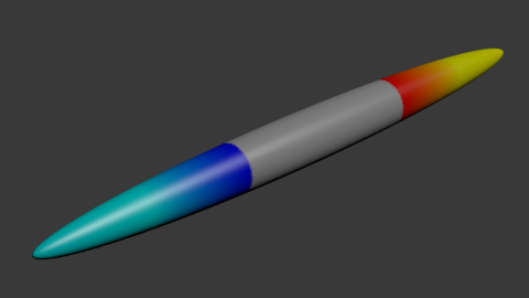
Example E

Here the data between -2 and 2 is used for scaling, but only the points between -1 and 1 are shown. This is because the option dual was set as false. The values below -1 or above 1 receive the same colours as these numbers, because the coption was configured as true. Note that because all points will receive some colour, it is not necessary to define the colourgap.

dpx2map ellipsoid-y.dpv ellipsoid.srf exE coolhot5 '[-2 2]' '[-1 1]' false '[]' true

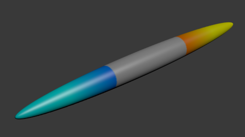
Example F

This is similar as the previous example, except that the values between -1 and 1 receive a colour off of the colour map. This is because both dual and coption were set as false.

dpx2map ellipsoid-y.dpv ellipsoid.srf exF coolhot5 '[-2 2]' '[-1 1]' false '[.75 .75 .75]' false

Facewise data

The process to display facewise data is virtually identical. The only two differences are that (1) instead of supplying a *.dpv file, a *.dpf file is given to the script as input, and (2) the output isn’t a *.ply file, but instead a pair of files *.obj + *.mtl. Note that very few software can handle thousands of colours per object in the case of facewise data. Blender is recommended over most commercial products specially for this reason (and of course, it is free, as in freedom).

Download

The dpx2map is available here, and it is also included in the areal package, described here, where all its dependencies are satisfied. You must have Octave (free) or Matlab available to use this tool.

How to cite

If you use dpx2map for your scientific research, please, remember to mention the brainder.org website in your paper.

Update: Display in PDF documents

3D models as these, with vertexwise colours, can be shown in interactive PDF documents. Details here.

Say you have a number of meshes in FreeSurfer ascii format (with extension *.asc or *.srf), one brain structure per file. However, for later processing or to import in some computer graphics software, you would like to have these multiple meshes all in a single file. This post provides a small script to accomplish this: mergesrf.

To use it, right click and save the file above, make it executable and, ideally, put it in a place where it can be found (or add its location to the environmental variable ${PATH}. Then run something as:

mergesrf file1.srf file2.srf fileN.srf mergedfile.srf

In this example, the output file is saved as mergedfile.srf. Another example is to convert all subcortical structures into just one large object, after aseg2srf as described here. To convert all, just change the current directory to ${SUBJECTS_DIR}//ascii, then run:

mergesrf * aseg_all.srf

A list with the input files and the output at the end is shown below:

The script uses Octave, which can be downloaded freely. The same script, with a small modification, can also run from inside matlab. This other version can be downloaded here: mergesrf.m

Requirements

In addition to Octave (or matlab), the script also requires functions to read and write surface files, which are available from the areal package (described here and downloadable here).