
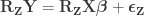
Doing a permutation test with the general linear model (GLM) in the presence of nuisance variables can be challenging. Let the model be:
where 


Because the interest is in testing the relationship between
One of these various methods is the one published in Freedman and Lane (1983), which consists of permuting data that has been residualised with respect to the covariates, then estimated covariate effects added back, then the full model fitted again. The procedure can be performed through the following steps:
- Regress
. Use the estimated parameters
to compute the statistic of interest, and call this statistic
.
- Regress
, obtaining estimated parameters
and estimated residuals
.
- Compute a set of permuted data
. This is done by pre-multiplying the residuals from the reduced model produced in the previous step,
, then adding back the estimated nuisance effects, i.e.
.
- Regress the permuted data
- Use the estimated
to compute the statistic of interest. Call this statistic
.
- Repeat the Steps 2-4 many times to build the reference distribution of
under the null hypothesis of no association between
- Count how many times

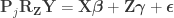
Steps 1-4 can be written concisely as:

where 


In page 385 of Winkler et al. (2014), my colleagues and I state that:
[…] add the nuisance variables back in Step 3 is not strictly necessary, and the model can be expressed simply as
, implying that the permutations can actually be performed just by permuting the rows of the residual-forming matrix
.
However, in the paper we do not offer any proof of this important result, that allows algorithmic acceleration. Here we remedy that. Let’s start with two brief lemmata:
Lemma 1: The product of a hat matrix and its corresponding residual-forming matrix is zero, that is, 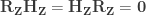
This is because 
Lemma 2 (Frisch–Waugh–Lovell theorem): Given a GLM expressed as 

To see why, remember that multiplying both sides of an equation by the same factor does not change it (least squares solutions may change; transformations using Lemma 2 below do not act on the fitted model). Let’s start from:

Then remove the parentheses:

Since

and that 

Since 

where 
Main result
Now we are ready for the main result. The Freedman-Lane model is:
Per Lemma 2, it can be rewritten as:

Dropping the parenthesis:

Per Lemma 1:


What is left has the same form as the result of Lemma 2. Thus, reversing it, we obtain the final result:
Hence, the hat matrix 
References
- Anderson MJ, Legendre P. An empirical comparison of permutation methods for tests of partial regression coefficients in a linear model. Journal of Statistical Computation and Simulation 1999;62(3):271–303.
- Anderson MJ, Robinson J. Permutation tests for linear models. Australian & New Zealand Journal of Statistics of Statistics 2001;43(1):75–88.
- Freedman D, Lane D. A Nonstochastic Interpretation of Reported Significance Levels. Journal of Business & Economic Statistics 1983;1(4):292.
- Winkler AM, Ridgway GR, Webster MA, Smith SM, Nichols TE. Permutation inference for the general linear model. NeuroImage 2014;92:381–97.
Updates
- 07.Jun.2020: A graphical representation of Lemma 1 can be found in p.40 of Jaromil Frossard PhD thesis (Université de Genève), available here.
- 07.Jun.2020: Lemma 2 corresponds to the Frisch–Waugh–Lovell theorem. Thanks to Samuel Davenport (University of Oxford) for pointing out.

 is the
  vector of observations,
  is the
  matrix of explanatory variables,
  is the
  vector of regression coefficients, and
  , where
  is a
is a  matrix that defines a contrast of regression coefficients, satisfying
  and
and  .
.
 vector of observations,
  is the
  vector of regression coefficients, and
  , where
  is a
is a  matrix that defines a contrast of observed variables, satisfying
  and
and  .
.

 and
and  .
.
 , the multiple correlation coefficient can be computed from the
  statistic as:
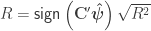
 statistic can be computed as:
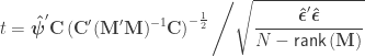
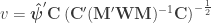
 statistic can be computed as:
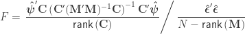
 is a diagonal matrix that has elements:
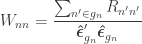
 are the
  diagonal elements of the residual forming matrix
  , and
, and  is the variance group to which the
  -th observation belongs.
 , is given by:
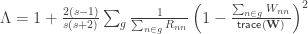

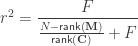
 is known, the formula can be solved for

![\mathbf{A} = \left[\mathbf{y}\; \mathbf{M}\right]](https://s0.wp.com/latex.php?latex=%5Cmathbf%7BA%7D+%3D+%5Cleft%5B%5Cmathbf%7By%7D%5C%3B+%5Cmathbf%7BM%7D%5Cright%5D&bg=ffffff&fg=333333&s=0&c=20201002) , and
, and  be the inverse of the correlation matrix of the columns of
  , and
, and  the diagonal operator, that returns a column vector with the diagonal entries of a square matrix. Then the matrix with the partial correlations is:
 is the
  ” is taken elementwise (i.e., not matrix power).
 as the sums of the products of the residuals, and
  as the sums of products of the hypothesis. In fact, the original model can be modified as
  , where
  ,
,  and
and  .
. , this is an univariate model, otherwise it remains multivariate, although
  and
and  .
. statistic can be computed as:


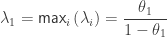
 be the eigenvalues of
  the eigenvalues of
  . Then:
 .
. .
. .
. (analogous to
  (analogous to
  is the
  -th canonical correlation.