In the previous post, the procedures to compute a statistic for six common normality tests and how to obtain the respective p-values using asymptotic approximations were briefly reviewed. In this post, it is shown that these approximations, that appear in classic statistical textbooks and papers, are not entirely accurate for arbitrary sample sizes or nominal levels of significance.
For each test, 1,000,000 realisations of normal distributions were simulated using matlab, computed analytically the p-values, and plotted their frequencies at significance intervals of 0.01, with 34 different sample sizes, ranging from 10 to 10,000 (more specifically: 10, 15, 20, 25, 30, 40, 50, 60, 70, 80, 90, 100, 150, 200, 250, 300, 400, 500, 600, 700, 800, 900, 1000, 1500, 2000, 2500, 3000, 4000, 5000, 6000, 7000, 8000, 9000, 10000). The best approximations should produce flat series of bars between p-values 0-1, and be stable across sample sizes, particularly at the most common significance levels: near or below p=0.05.
In general, any test can be analysed according to power, robustness to sample size, ability to correctly reject some specific types of distributions and other parameters. The analyses presented here refer exclusively to the ability to reject the null when the null is true at the nominal significance level using analytical approximations. Poor performance in this analysis does not imply that the test, per se, is poor. It only implies that the approximation used to derive the p-values is not accurate. The tests may still be very powerful to detect non-normality, but accurate p-values must then rely on tables produced via Monte Carlo simulations, which are, by definition, always exact.
Skewness test
The skewness test is perhaps the one that performed better in terms of asymptotic approximation to a p-value (which does not imply that this test is at all more powerful or has any other feature that would qualify it as better than the others). The approximation produces p-values that are virtually identical to the nominal p-values for any of the sample sizes.
")
")
")
Kurtosis test
The asymptotic approximation for the kurtosis test performed reasonably well for most significance levels and for large sample sizes. However, it produced an excess of low p-values for sample sizes smaller than 20, implying that the test can be anti-conservative with small samples.
")
")
")
D’Agostino-Pearson omnibus test
The p-value approximation for the D’Agostino-Pearson  statistic had a poor and erratic behaviour for sample sizes smaller than 200, particularly at the low significance levels, which are generally the ones of greatest interest. For this test, Monte Carlo simulations to derive the critical values are highly recommended.
")
")
")
Jarque-Bera test
Another test for which the asymptotic approximation was poor is the Jarque-Bera test. The approximation to the distribution of the  statistic is not valid for small p-values for any of the sample sizes tested, although for sample sizes >1500 the behaviour was reasonably stable. Monte Carlo simulations also more appropriate for this test.
")
")
")
Shapiro-Wilk test
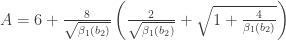
The asymptotic approximation to the distribution of the Shapiro-Wilk’s  statistic seems adequate for sample sizes larger than 15 and smaller than 4000, being slightly anticonservative for most p-values at sample sizes smaller than 20. It has aberrant behaviour at p-values close to 1, which are generally of no interest anyway.
")
")
")
Shapiro-Francia test
For the Shapiro-Francia’s  statistic, the asymptotic behaviour is similar to the observed for the Shapiro-Wilk test, except that it remains valid for sample sizes larger than 4000.
")
")
")
Other tests
Other popular normality or distributional tests, such as the Kolmogorov-Smirnov test, the Lilliefors test, the Cramér-von Mises criterion or the Anderson-Darling test, do not have well established asymptotic approximations and, as a consequence, depend on Monte Carlo simulations to derive critical values. The p-values for these tests are always accurate, as long as the simulations were performed adequately.
Conclusion
Care should be taken when using formulas that approximate the distribution for the statistic for these tests. The approximations are not perfectly valid for all sample sizes, and can be very inaccurate in many cases. When in doubt, critical values based on Monte Carlo tests might be preferred.


 is the transformed value for observation
  ,
,  is the
  is the ordinary rank of the
  observations.
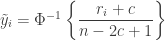
 is a constant and the remaining variables are as above. The value of
  , Tukey (1962) suggests
  , Bliss (1967) suggests
  and, as just decribed, Van der Waerden suggests
  .
.


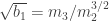 , where
 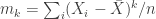 is the k-th moment,
  is the sample mean, and


 is the test statistic and it is approximately normally distributed under the null hypothesis that the population data follows a normal distribution.
 , where


 , where
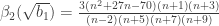
  and
and  represent respectively the expected value and the variance.
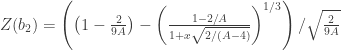
 is the test statistic and is considered approximately normally distributed under the null hypothesis that the population data follows a normal distribution.
 . In other words, simply square the statistics from the skewness and kurtosis tests and sum them together. The distribution of the
  distribution with two degrees of freedom under the null hypothesis that the sample was drawn from a population with normally distributed values. The skewness, kurtosis and the D’Agostino-Pearson tests have been collectively reviewed and discussed in
  . The
. The  is asymptotically distributed as a
  , where
  represents the inverse normal cdf.
 . These weights are the same used in the Shapiro-Francia test (see below).
 , where
  . If
. If  , compute also
  .
. if
if  or
or  otherwise.
 for
for  if
if  if
if  .
. to a normal distribution with mean
  and standard deviation
  (
( , where
  . For sample sizes equal to or larger than 12,
  .
. , the parameters of the statistic transformed (normalized) by
  and
and  . For
. For  ,
,  and
and  , where
  .
. statistic can then be produced trivially by
  , and the p-values can be obtained from the normal cdf.
 .
. to a normal distribution with mean
  are given by
  , where
  and
and  , where
  . These approximations are valid for samples between 5 and 5000 at least.
 , and the p-values can be obtained from the normal cdf.