April | 2012 | Brainder.

A Bernoulli trial is an experiment in which the outcome can be one of two mutually exclusive results, e.g. true/false, success/failure, heads/tails and so on. A number of methods are available to compute confidence intervals after many such trials have been performed. The most common have been discussed and reviewed by Brown et al. (2001), and are presented below. Consider $n$ trials, with $X$ successes and a significance level of $\alpha=0.05$ to obtain a 95% confidence interval. For each of the methods, the interval is shown graphically for $1 \leqslant n \leqslant 100$ and $1 \leqslant X \leqslant n$ .

Wald

This is the most common method, discussed in many textbooks, and probably the most problematic for small samples. It is based on a normal approximation to the binomial distribution, and it is often called “Wald interval” for it’s relationship with the Wald test. The interval is calculated as:

Lower bound: $L=p-k\sqrt{pq/n}$
Upper bound: $U=p+k\sqrt{pq/n}$

where $k = \Phi^{-1}\{1-\alpha/2\}$ , $\Phi^{-1}$ is the probit function, $p=X/n$ and $q=1-p$ .

Wald confidence interval.

Wilson

This interval appeared in Wilson (1927) and is defined as:

Lower bound: $L = \tilde{p} - (k/\tilde{n})\sqrt{npq+k^2/4}$
Upper bound: $U = \tilde{p} + (k/\tilde{n})\sqrt{npq+k^2/4}$

where $\tilde{p} = \tilde{X}/\tilde{n}$ , $\tilde{n}=n+k^2$ , $\tilde{X} = X+ k^2/2$ , and the remaining are as above. This is probably the most appropriate for the majority of situations.

Wilson confidence interval.

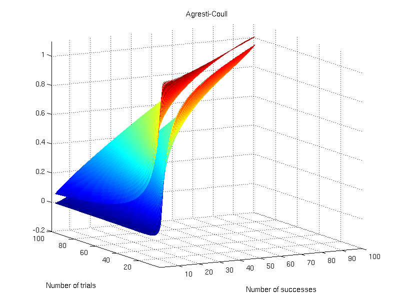
Agresti-Coull

This interval appeared in Agresti and Coull (1998) and shares many features with the Wilson interval. It is defined as:

Lower bound: $L = \tilde{p} - k\sqrt{\tilde{p}\tilde{q}/\tilde{n}}$
Upper bound: $U = \tilde{p} + k\sqrt{\tilde{p}\tilde{q}/\tilde{n}}$

where $\tilde{q}=1-\tilde{p}$ , and the remaining are as above.

Agresti-Coull confidence interval.

Jeffreys

This interval has a Bayesian motivation and uses the Jeffreys prior (Jeffreys, 1946). It seems to have been introduced by Brown et al. (2001). It is defined as:

Lower bound: $L = \mathcal{B}^{-1}\{\alpha/2,X+1/2,n-X+1/2\}$
Upper bound: $U = \mathcal{B}^{-1}\{1-\alpha/2,X+1/2,n-X+1/2\}$

where $\mathcal{B}^{-1}\{x,s_1,s_2\}$ is the inverse cdf of the beta distribution (not to be confused with the beta function), at the quantile $x$ , and with shape parameters $s_1$ and $s_2$ .

Jeffreys confidence interval.

Clopper-Pearson

This interval was proposed by Clopper and Pearson (1934) and is based on a binomial test, rather than on approximations, hence sometimes being called “exact”, although it is not “exact” in the common sense. It is considered overly conservative.

Lower bound: $L = \mathcal{B}^{-1}\{\alpha/2,X,n-X+1\}$
Upper bound: $U = \mathcal{B}^{-1}\{1-\alpha/2,X+1,n-X\}$

where $\mathcal{B}^{-1}\{x,s_1,s_2\}$ is the inverse cdf of the beta distribution as above.

Clopper-Pearson confidence interval.

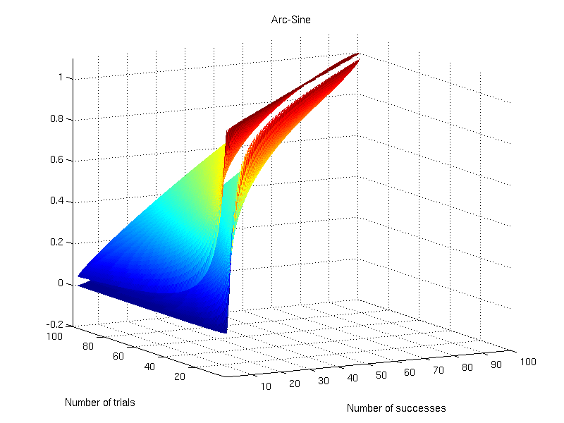
Arc-Sine

This interval is based on the arc-sine variance-stabilising transformation. The interval is defined as:

Lower bound: $L = \sin\{\arcsin\{\sqrt{a}\} - k/(2\sqrt{n})\}^2$
Upper bound: $U = \sin\{\arcsin\{\sqrt{a}\} + k/(2\sqrt{n})\}^2$

where $a=\frac{X+3/8}{n+3/4}$ replaces what otherwise would be $p$ (Anscombe, 1948).

Arc-sine confidence interval.

Logit

This interval is based on the Wald interval for $\lambda = \ln\{\frac{X}{n-X}\}$ . It is defined as:

Lower bound: $L = e^{\lambda_L}/(1+e^{\lambda_L})$
Upper bound: $U = e^{\lambda_U}/(1+e^{\lambda_U})$

where $\lambda_L = \lambda - k\sqrt{\hat{V}}$ , $\lambda_U = \lambda + k\sqrt{\hat{V}}$ , and $\hat{V} = \frac{n}{X(n-X)}$ .

Logit confidence interval.

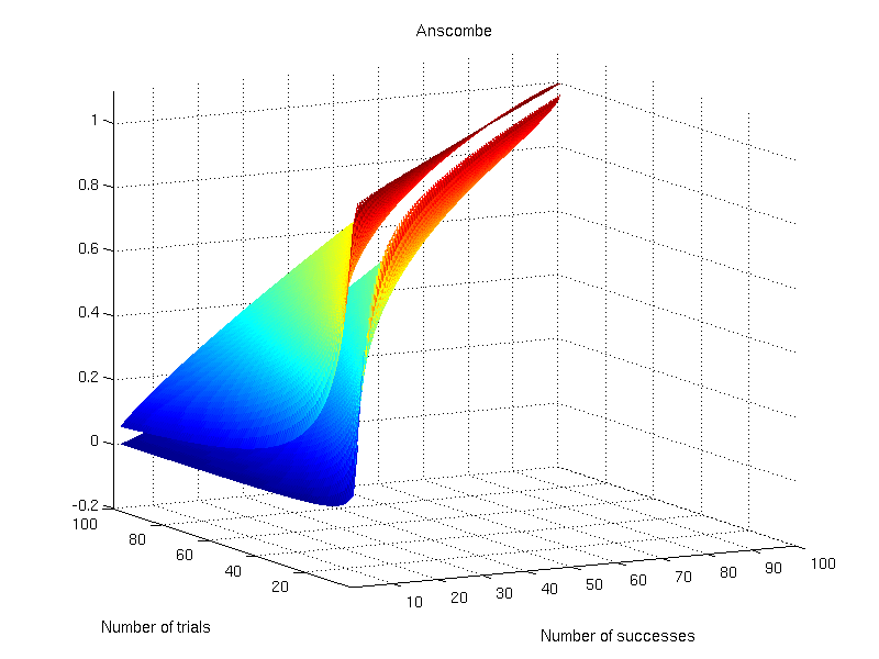
Anscombe

This interval was proposed by Anscombe (1956) and is based on the logit interval:

Lower bound: $L = e^{\lambda_L}/(1+e^{\lambda_L})$
Upper bound: $U = e^{\lambda_U}/(1+e^{\lambda_U})$

The difference is that $\lambda=\ln\{\frac{X+1/2}{n-X+1/2}\}$ and $\hat{V}=\frac{(n+1)(n+2)}{n(X+1)(n-X+1)}$ . The values for $\lambda_L$ and $\lambda_U$ are as above.

Anscombe’s confidence interval.

Octave/MATLAB implementation

A function that computes these intervals is available here: confint.m.

References

Agresti A and Coull BA. Approximate is better than “exact” for interval estimation of binomial proportions. The American Statistician. 1998; 52(2):119-126.
Anscombe FJ The transformation of Poisson, binomial and negative-binomial data. Biometrika. 1948; 35(3/4:246-254.
Anscombe FJ. On estimating binomial response relations. Biometrika. 1956; 43(3/4):461-464.
Brown LD, Cai TT, DasGupta A. Interval estimation for a binomial proportion. Statist Sci. 2001; 16(2):101-133.
Clopper CJ, Pearson ES. The use of confidence or fiducial limits illustrated in the case of the binomial. Biometrika. 1934; 26(4):404-413.
Jeffreys H. An invariant form for the prior probability in estimation problems. Proc. R. Soc. Lond. A. 1946; 186(1007):453-461.
Wilson EB. Probable inference, the law of succession, and statistical inference. J Am Stat Assoc. 1927; 22(158):209-21.

Main file

The links to the script are below. Either of these will work; choose according to your needs:

platonic – This is the Octave script. Simply download it, change the first line to point to your correct Octave location, make it executable, and run it directly from the shell. Call it without arguments to obtain usage information.

platonic.m – This is the same as above, but can be executed from within Octave or MATLAB. Type ‘help platonic’ to obtain usage information.

Examples

To create an icosahedron with radius 100, recursively subdivided 7 times, if from the shell, use:

platonic ico7.obj ico sph 7 100

or, if from inside Octave/MATLAB, use:

platonic('ico7.obj','ico','sph',7,100);

The outputs from platonic are always in Wavefront (.obj) format. To use this icosahedron, e.g., with areal interpolation, it needs to be converted to FreeSurfer ascii format:

obj2srf ico7.obj > ico7.srf

The obj2srf command is available in the package for areal analysis, here.

References

Kenner H. Geodesic math and how to use it. University of California Press, Los Angeles, USA, 1976.

Winkler AM, Sabuncu MR, Yeo BT, Fischl B, Greve DN, Kochunov P, Nichols TE, Blangero J, Glahn DC. Measuring and comparing brain cortical surface area and other areal quantities. Neuroimage. 2012 Jul 16;61(4):1428-43