March | 2015 | Brainder.

It’s so often that we find ourselves in the need to quickly compute a statistic for a certain dataset, but finding the formulas is not always direct. Using a statistical software is helpful, but it often also happens that the reported results are not exactly what one may believe it represents. Moreover, even if using these packages, it is always good to have in mind the meaning of statistics and how they are computed. Here the formulas for the most commonly used statistics with the general linear model (glm) are presented, all in matrix form, that can be easily implemented in Octave or Matlab.

I — Model

We consider two models, one univariate, another multivariate. The univariate is a particular case of the multivariate, but for univariate problems, it is simpler to use the smaller, particular case.

Univariate model

The univariate glm can be written as:

$\mathbf{y} = \mathbf{M}\boldsymbol{\psi} + \boldsymbol{\epsilon}$

where $\mathbf{y}$ is the $N \times 1$ vector of observations, $\mathbf{M}$ is the $N \times s$ matrix of explanatory variables, $\boldsymbol{\psi}$ is the $s \times 1$ vector of regression coefficients, and $\boldsymbol{\epsilon}$ is the $N \times 1$ vector of residuals.

The null hypothesis can be stated as $\mathcal{H}_0 : \mathbf{C}'\boldsymbol{\psi} = 0$ , where $\mathbf{C}$ is a $s \times s'$ matrix that defines a contrast of regression coefficients, satisfying $\mathsf{rank}(\mathbf{C}) = s'$ and $1 \geqslant s' \geqslant s$ .

Multivariate model

The multivariate glm can be written as:

$\mathbf{Y} = \mathbf{M}\boldsymbol{\Psi} + \boldsymbol{\epsilon}$

where $\mathbf{Y}$ is the $N \times q$ vector of observations, $\mathbf{M}$ is the $N \times s$ matrix of explanatory variables, $\boldsymbol{\Psi}$ is the $s \times q$ vector of regression coefficients, and $\boldsymbol{\epsilon}$ is the $N \times q$ vector of residuals.

The null hypothesis can be stated as $\mathcal{H}_0 : \mathbf{C}'\boldsymbol{\Psi}\mathbf{D} = 0$ , where $\mathbf{C}$ is defined as above, and $\mathbf{D}$ is a $q \times q'$ matrix that defines a contrast of observed variables, satisfying $\mathsf{rank}(\mathbf{D}) = q'$ and $1 \geqslant q' \geqslant q$ .

II — Estimation of parameters

In the model, the unknowns of interest are the values arranged in $\boldsymbol{\Psi}$ . These can be estimated as:

$\boldsymbol{\hat{\Psi}} = (\mathbf{M}'\mathbf{M})^{+}(\mathbf{M}'\mathbf{Y})$

where the $^{+}$ represents a pseudo-inverse. The residuals can be computed as:

$\boldsymbol{\hat{\epsilon}} = \mathbf{Y} - \mathbf{M}\boldsymbol{\hat{\Psi}}$

The above also applies to the univariate case ( $\mathbf{y}$ is a particular case of $\mathbf{Y}$ , and $\boldsymbol{\psi}$ of $\boldsymbol{\Psi}$ ).

III – Univariate statistics

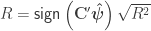
Coefficient of determination, R²

The following is the fraction of the variance explained by the part of the model determined by the contrast. It applies to mean-centered data and design, i.e., $\tilde{\mathbf{y}}=\mathbf{y}-\bar{y}$ and $\tilde{\mathbf{M}}=\mathbf{M}-\bar{\mathbf{m}}$ .

$R^2 = \dfrac{\boldsymbol{\hat{\psi}}'\mathbf{C} \left(\mathbf{C}'(\tilde{\mathbf{M}}'\tilde{\mathbf{M}})^{-1}\mathbf{C} \right)^{-1} \mathbf{C}'\boldsymbol{\hat{\psi}}}{\tilde{\mathbf{y}}'\tilde{\mathbf{y}}}$

Note that the portion of the variance explained by nuisance variables (if any) remains in the denominator. To have these taken into account, consider the squared partial correlation coefficient, or Pillai’s trace with univariate data, both described further down.

Pearson’s correlation coefficient

When $\mathsf{rank}\left(\mathbf{C}\right) = 1$ , the multiple correlation coefficient can be computed from the $R^2$ statistic as:

$R = \mathsf{sign}\left(\mathbf{C}'\boldsymbol{\hat{\psi}}\right)\sqrt{R^2}$

This value should not be confused, even in the presence of nuisance, with the partial correlation coefficient (see below).

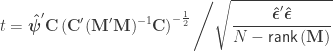
Student’s t statistic

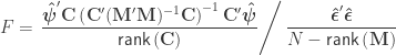
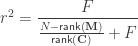
If $\mathsf{rank}\left(\mathbf{C}\right) = 1$ , the Student’s $t$ statistic can be computed as:

$t = \boldsymbol{\hat{\psi}}'\mathbf{C} \left(\mathbf{C}'(\mathbf{M}'\mathbf{M})^{-1}\mathbf{C} \right)^{-\frac{1}{2}} \left/ \sqrt{\dfrac{\boldsymbol{\hat{\epsilon}}'\boldsymbol{\hat{\epsilon}}}{N-\mathsf{rank}\left(\mathbf{M}\right)}} \right.$

F statistic

The $F$ statistic can be computed as:

$F = \left.\dfrac{\boldsymbol{\hat{\psi}}'\mathbf{C} \left( \mathbf{C}'(\mathbf{M}'\mathbf{M})^{-1}\mathbf{C} \right)^{-1} \mathbf{C}'\boldsymbol{\hat{\psi}}}{\mathsf{rank}\left(\mathbf{C} \right)} \right/ \dfrac{\boldsymbol{\hat{\epsilon}}'\boldsymbol{\hat{\epsilon}}}{N-\mathsf{rank}\left(\mathbf{M}\right)}$

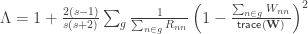
Aspin—Welch v

If homoscedastic variances cannot be assumed, and $\mathsf{rank}\left(\mathbf{C}\right) = 1$ , this is equivalent to the Behrens—Fisher problem, and the Aspin—Welch’s $t$ statistic can be computed as:

$v = \boldsymbol{\hat{\psi}}'\mathbf{C} \left(\mathbf{C}'(\mathbf{M}'\mathbf{W}\mathbf{M})^{-1}\mathbf{C} \right)^{-\frac{1}{2}}$

where $\mathbf{W}$ is a diagonal matrix that has elements:

$W_{nn}=\dfrac{\sum_{n' \in g_{n}}R_{n'n'}}{\boldsymbol{\hat{\epsilon}}_{g_{n}}'\boldsymbol{\hat{\epsilon}}_{g_{n}}}$

and where $R_{n'n'}$ are the $n'$ diagonal elements of the residual forming matrix $\mathbf{R} = \mathbf{I}-\mathbf{M}\mathbf{M}^{+}$ , and $g_{n}$ is the variance group to which the $n$ -th observation belongs.

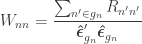
Generalised G statistic

If variances cannot be assumed to be the same across all observations, a generalisation of the $F$ statistic can be computed as:

$G = \dfrac{\boldsymbol{\hat{\psi}}'\mathbf{C} \left(\mathbf{C}'(\mathbf{M}'\mathbf{W}\mathbf{M})^{-1}\mathbf{C} \right)^{-1} \mathbf{C}'\boldsymbol{\hat{\psi}}}{\Lambda \cdot \mathsf{rank}\left(\mathbf{C}\right)}$

where $\mathbf{W}$ is defined as above, and the remaining denominator term, $\Lambda$ , is given by:

$\Lambda = 1+\frac{2(s-1)}{s(s+2)}\sum_{g} \frac{1}{\sum_{n \in g}R_{nn}} \left(1-\frac{\sum_{n \in g}W_{nn}}{\mathsf{trace}\left(\mathbf{W}\right)}\right)^2$

There is another post on the G-statistic (here).

Partial correlation coefficient

When $\mathsf{rank}\left(\mathbf{C}\right) = 1$ , the partial correlation can be computed from the Student’s $t$ statistic as:

$r = \mathsf{sign}\left(t\right)\sqrt{\dfrac{t^2}{N-\mathsf{rank}\left(\mathbf{M}\right)+t^2}}$

The square of the partial correlation corresponds to Pillai’s trace applied to an univariate model, and it can also be computed from the $F$ -statistic as:

$r^2 = \dfrac{F}{\frac{N-\mathsf{rank}\left(\mathbf{M}\right)}{\mathsf{rank}\left(\mathbf{C}\right)}+F}$

Likewise, if $r$ is known, the formula can be solved for $t$ :

$t = \dfrac{r\sqrt{N-\mathsf{rank}\left(\mathbf{M}\right)}}{\sqrt{1-r^2}}$

or for $F$ :

$F = \dfrac{r^2}{1-r^2}\times\dfrac{N-\mathsf{rank}\left(\mathbf{M}\right)}{\mathsf{rank}\left(\mathbf{C}\right)}$

The partial correlation can also be computed at once for all variables vs. all other variables as follows. Let $\mathbf{A} = \left[\mathbf{y}\; \mathbf{M}\right]$ , and $\mathsf{r}\left(\mathbf{A}\right)$ be the inverse of the correlation matrix of the columns of $\mathbf{A}$ , and $\mathsf{d}\left(\cdot\right)$ the diagonal operator, that returns a column vector with the diagonal entries of a square matrix. Then the matrix with the partial correlations is:

$\mathbf{r} = -\mathsf{r}\left(\mathbf{A}\right) \odot \left(\mathsf{d}\left(\mathsf{r}\left(\mathbf{A}\right)\right)\mathsf{d}\left(\mathsf{r}\left(\mathbf{A}\right)\right)'\right)^{-\frac{1}{2}}$

where $\odot$ is the Hadamard product, and the power “ $-\frac{1}{2}$ ” is taken elementwise (i.e., not matrix power).

IV – Multivariate statistics

For the multivariate statistics, define generically $\mathbf{E} = (\boldsymbol{\hat{\epsilon}}\mathbf{D})'(\boldsymbol{\hat{\epsilon}}\mathbf{D})$ as the sums of the products of the residuals, and $\mathbf{H}=(\mathbf{C}'\boldsymbol{\hat{\Psi}}\mathbf{D})' \left(\mathbf{C}'(\mathbf{M}'\mathbf{M})^{-1}\mathbf{C} \right)^{-1} (\mathbf{C}'\boldsymbol{\hat{\Psi}}\mathbf{D})$ as the sums of products of the hypothesis. In fact, the original model can be modified as $\tilde{\mathbf{Y}} = \mathbf{M}\tilde{\boldsymbol{\Psi}} + \tilde{\boldsymbol{\epsilon}}$ , where $\tilde{\mathbf{Y}}=\mathbf{Y}\mathbf{D}$ , $\tilde{\boldsymbol{\Psi}} = \boldsymbol{\Psi}\mathbf{D}$ and $\tilde{\boldsymbol{\epsilon}}=\boldsymbol{\epsilon}\mathbf{D}$ .

If $\mathsf{rank}\left(\mathbf{D}\right)=1$ , this is an univariate model, otherwise it remains multivariate, although $\mathbf{D}$ can be omitted from the formulas. From now on this simplification is adopted, so that $\mathbf{E} = \boldsymbol{\hat{\epsilon}}'\boldsymbol{\hat{\epsilon}}$ and $\mathbf{H}=\boldsymbol{\hat{\Psi}}'\mathbf{C} \left(\mathbf{C}'(\mathbf{M}'\mathbf{M})^{-1}\mathbf{C} \right)^{-1} \mathbf{C}'\boldsymbol{\hat{\Psi}}$ .

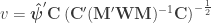
Hotelling T²

If $\mathsf{rank}\left(\mathbf{C}\right) = 1$ , the Hotelling’s $T^2$ statistic can be computed as:

$T^2 = \mathbf{C}'\boldsymbol{\hat{\Psi}}\boldsymbol{\Sigma}^{-\frac{1}{2}}\left(\mathbf{C}'(\mathbf{M}'\mathbf{M})^{-1}\mathbf{C} \right)^{-1}\boldsymbol{\Sigma}^{-\frac{1}{2}} \boldsymbol{\hat{\Psi}}'\mathbf{C}$

where $\boldsymbol{\Sigma} = \mathbf{E}/\left(N-\mathsf{rank}\left(\mathbf{M}\right)\right)$

Multivariate alternatives to the F statistic

Classical manova/mancova statistics can be based in the ratio between the sums of products of the hypothesis and the sums of products of the residuals, or the ratio between the sums of products of the hypothesis and the total sums of products. In other words, define:

$\begin{array}{ccl} \mathbf{A} &=& \mathbf{H}\mathbf{E}^{-1} = \mathbf{E}^{-\frac{1}{2}} \boldsymbol{\hat{\psi}}'\mathbf{C} \left(\mathbf{C}'(\mathbf{M}'\mathbf{M})^{-1}\mathbf{C} \right)^{-1} \mathbf{C}'\boldsymbol{\hat{\psi}}\mathbf{E}^{-\frac{1}{2}}\\ \mathbf{B} &=& \mathbf{H}\left(\mathbf{E}+\mathbf{H}\right)^{-1} \end{array}$

Let $\lambda_i$ be the eigenvalues of $\mathbf{A}$ , and $\theta_i$ the eigenvalues of $\mathbf{B}$ . Then:

Wilks’ $\Lambda = \prod_{i} \dfrac{1}{1+\lambda_i} = \dfrac{|\mathbf{E}|}{|\mathbf{E}+\mathbf{H}|}$ .
Lawley–Hotelling’s trace: $\sum_i \lambda_i = \mathsf{trace}\left(\mathbf{A}\right)$ .
Pillai’s trace: $\sum_i \dfrac{\lambda_i}{1+\lambda_i} = \sum_i \theta_i = \mathsf{trace}\left(\mathbf{B}\right)$ .
Roy’s largest root (ii): $\lambda_1 = \mathsf{max}_i\left(\lambda_i\right) = \dfrac{\theta_1}{1-\theta_1}$ (analogous to $F$ ).
Roy’s largest root (iii): $\theta_1 = \mathsf{max}_i\left(\theta_i\right) = \dfrac{\lambda_1}{1+\lambda_1}$ (analogous to $R^2$ ).

When $\mathsf{rank}\left(\mathbf{C}\right) = 1$ , or when $\mathbf{Y}$ is univariate, or both, Lawley–Hotelling’s trace is equal to Roy’s (ii) largest root, Pillai’s trace is equal to Roy’s (iii) largest root, and Wilks’ $\Lambda$ added to Pillai’s trace equals to unity. The value $\rho_i=\sqrt{\theta_i}$ is the $i$ -th canonical correlation.

References

- Wilks S. Certain Generalizations in the Analysis of Variance. Biometrika. 1932;24(3):471-494.
- Lawley D. A Generalization of Fisher’s z Test. Biometrika. 1938;30(1):180-187.
- Hotelling H. A generalized T test and measure of multivariate dispersion. In: Neyman J, ed. Proceedings of the Second Berkeley Symposium on Mathematical Statistics and Probability. Berkeley: University of California Press; 1951:23-41.
- Roy SN. On a Heuristic Method of Test Construction and its use in Multivariate Analysis. Ann Math Stat. 1953;24(2):220-238.
- Pillai KCS. Some New Test Criteria in Multivariate Analysis. Ann Math Stat. 1955;26(1):117-121.
- Winkler AM, Ridgway GR, Webster MA, Smith SM, Nichols TE. Permutation Inference for the general linear model. Neuroimage. 2014 May 15;92:381-97.