We often think of statistics as a way to summarize large amounts of data. For example, we can collect data from thousands of subjects, and extract a single number that tells something about these subjects. The well known German tank problem shows that, in a certain way, statistics can also be used for the opposite: using incomplete data and a few reasonable assumptions (or real knowledge), statistics provides way to estimate information that offer a panoramic view of all the data. Historical problems are interesting on their own. Yet, it is not always that we see so clearly consequential historical events at the time they happen — like now.
In the Second World War, as in any other war, information could be more valuable than anything else. Intelligence reports (such as from spies) would feed the Allies with information about the industrial capacity of Nazi Germany, including details about things such as the number of tanks produced. This kind of information can have far reaching impact and not only determine the outcome of a battle, but also if a battle would even even happen or with what preparations, as the prospect of finding a militarily superior opponent is often a great deterrent.
Sometimes, German tanks, as the well known Panzer, could be captured and carefully inspected. Among the details noted were the serial number printed in various pieces, such as chassis, gearboxes, and the serial numbers of the moulds used to produce the wheels. With the serial number of even a single chassis, for example one can estimate the total number of tanks produced; knowing the serial number of a single wheel mould allows the estimation of the total number of moulds, and thus, how many wheels can be produced in a certain amount of time. But how?
If serial numbers are indeed serial, e.g.,  , growing uniformly and without gaps, and we see a tank that has a serial number
  , then clearly at least tanks must have been produced. But could we have a better guess?
Let’s start by reversing the problem: suppose we knew  . In that case, what would be the average value of the serial numbers of all tanks? The average for uniformly distributed data like this would be
  , that is, the average of the first and last serial numbers.
Now, say we have only one sighting of a tank, and that has serial number . Then our best guess for the average serial number is itself, as we have no additional information. Thus, with  , our guess would be
  (that is, reorganizing the terms of the previous equation for
  ). Note that, for one sighting, this formula guarantees that is larger or equal than , which makes sense: we cannot have an estimate for that is smaller than the serial number itself.
What if we had not just one, but multiple sightings? Call the number of sightings  . The mean is now
 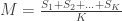 , for ordered serial numbers
  . Clearly, we can’t use the same formula, because if is much smaller than
  (say, because we have seen many small serial numbers, but just a handful of larger ones), could incorrectly be estimated as less than , which makes no sense. At least tanks must exist.
While incorrect for  , the above formula gives invaluable insight: it shows that for such uniformly distributed data, approximately half of the tanks have serial number above , the other half below . Extending the idea, and still under the assumption that the serial numbers are uniform, we can conclude that the number of tanks below the lowest serial number
  (which is
  ) must be approximately the same as the (unknown) number of tanks above the highest serial number . So, a next better estimate could be to use
  .
.
We can still do better, though. Since we have sightings, we can estimate what is the average interval between sightings, i.e.,  . As it is based on all sightings, this gives a better estimate of the spacing between the serial numbers than the single sighting . The result can be added to . The final estimate then becomes
  .
.
To make this concrete, say we saw tanks numbered  . Then our best guess would be
  .
.
At the end of the war, estimates obtained using the above method proved remarkably accurate, much more so than information provided by spies and other intelligence reports.
Let’s now see a similar example that is contemporary to us. Take the current pandemic caused by a novel coronavirus. The World Health Organization stated officially, in 14th January 2020, when there were 41 cases officially reported in China, that there was no evidence for human-to-human transmission. Yet, when the first 3 cases outside China were confirmed in 16th January 2020, epidemiologists at the Imperial College London were quick to find out that the WHO statement must have not been true. Rather, the real number of cases was likely well above 1700.
How did they make that estimate? The key insight was the realisation that only a small number of people in any major city travels internationally, particularly in such a short time span like that given by the time until the onset of symptoms for this kind of respiratory disease. If one can estimate prevalence among those who travelled, that would be a good approximation to the prevalence among those who live in the city, assuming that those who travel are an unbiased sample of the population.
Following this idea, we have:  , that is, the number of cases among those who travelled (
 ) divided by the total number of people who travelled (
 ) is expected to be approximately the same as the number of cases among those who stayed (
 ) divided by the total number of people who stayed (live) in the city (
 ).
).
The number of people served by the international airport of Wuhan is about 19 million (the size of the Wuhan metropolitan area), and the average daily number of outbound international passengers in previous years was 3301 for that time of the year (a figure publicly known, from IATA). Unfortunately, little was known outside China about the time taken between exposure to the virus and the onset of symptoms. The researchers then resorted to a proxy: the time known for the related severe respiratory disorder known as MERS, also caused by a coronavirus, which is about 10 days. Thus, we can estimate  people travelling out, and
  staying in the city. The number of known international cases was at the time
  . Hence:
 cases
cases
So, using remarkably simple maths, simpler even than in our WWII German tank example, the scientists estimated that the number of actual cases in the city of Wuhan was likely far above the official figure of 41 cases. The researchers were careful to indicate that, should the probability of travelling be higher among those exposed, the number of actual cases could be smaller. The converse is true: should travellers be wealthier (thus less likely to be exposed to a possible zoonosis as initially reported), the number of actual cases could be higher.
Importantly, it is not at all likely that 1700 people would have contracted such a zoonosis from wild animals in a dense urban area like Wuhan, hence human-to-human transmission must had been occurring. Eventually the WHO confirmed human-to-human transmission on 19th January 2020. Two days later, Chinese authorities began locking down and sealing off Wuhan, thus putting into place a plan to curb the transmission.
To find out more about the original problem of the number of tanks, and also for other methods of estimation for the same problem, a good start is this article. Also invaluable, for various estimation problems related to the fast dissemination of the novel coronavirus, are all the reports by the epidemiology team at the Imperial College London, which can be found here.


. Use the estimated parameters
to compute the statistic of interest, and call this statistic
.
, obtaining estimated parameters
and estimated residuals
.
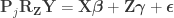
. This is done by pre-multiplying the residuals from the reduced model produced in the previous step,
, then adding back the estimated nuisance effects, i.e.
.
to compute the statistic of interest. Call this statistic
.
under the null hypothesis of no association between


, implying that the permutations can actually be performed just by permuting the rows of the residual-forming matrix
.