This post describes a reimplementation of the method described by Caruyer et al. (2013). If you already know what this is about, you can skip the information below and simply download the code from GitHub: multishell.py. If you don’t know, a good place to start is Tuch et al. (2004).
Background
When we plan a magnetic resonance imaging protocol, we often have to balance what we would like to have in terms of quantity and quality of images, versus what can realistically be obtained within limited time slots (e.g., 30 minutes or 1 hour) while minimizing discomfort to the research participants, most of whom would rather not spend more than an hour in a somewhat uncomfortable MRI exam table. For diffusion weighted imaging, we want as many directions in q-space as possible, and that the directions are uniformly sampled across all possible directions, which help subsequent modelling of various diffusion parameters, fiber orientation and fiber crossings.
In practice, we need to establish a set of directions that uniformly covers the surface of a sphere. Presets available within the scanner workstation, provided by the manufacturer, are sometimes helpful but these are not entirely customizable. For example, for Siemens scanners, the number of directions can be selected as 6, 10, 12, 20, 30, 64, 128, or 256. But what if the number of directions for your experiment that makes best use of the time available is none of these? The problem becomes more complicated if there are multiple b-values (e.g., in a multishell acquisition or, e.g., with diffusion spectrum imaging). How to find the directions that uniformly sample all possible directions, without repetitions across shells, and while taking into account the multiple b-values?
Note that this is not simply a matter of finding random points uniformly distributed on the surface of a sphere. That could be done by simply generating independent Gaussian noise in the 3D space, then scaling the distance of each point to the center of the coordinate system to a certain radius, e.g., 1 (that is, treating each point as a vector and scaling it to unit norm). Instead, what we want are directions that are as far apart from each other as possible, so that the resulting image for each provides maximally unique information.
Moreover, having an arbitrary number of points equally separated on the surface of a sphere is impossible. Only five configurations exist, with at most 20 points; these configurations correspond to vertex locations of the five Platonic polyhedra. We need, therefore, to be content with values that are as spaced as possible on the surface, already knowing they can’t be all equally spaced.
Cost function
For just one b-value (one shell), a possible solution is to treat each direction as a charged particle in the surface of a sphere centered at the center of the coordinate system. The positions of the particles can then be established such that the electrostatic repulsion forces are minimized (Conturo et al., 1996; Jones et al., 1999). Caruyer et al. (2013) extended the idea to multiple b-values (multiple shells). Using the same notation as in the original paper, consider 


The above takes into account the direct repulsion between the two particles (first term, with a difference in the denominator) as well as repulsion between their antipodal representations (second term, with a sum in the denominator). Caruyer et al. (2013) then go on to propose the following cost functions for intra-shell and inter-shell electrostatic forces:
Intra-shell uniformity: Minimizing intra-shell electrostatic repulsion forces ensures that the points (directions) within each shell are evenly spread (Equation 2 if the paper):

where 


Inter-shell uniformity: Minimizing inter-shell electrostatic repulsion forces ensures that points across all shells, when projected onto a unit sphere, are evenly spread (Equation 4 in the paper):

where 
We have therefore two cost-functions that can be combined with a suitable factor that gives more or less weight for repulsions within- or between-shells:

under the constraint that all points need to lie on the surface of a sphere of radius 1.
Gradient
The gradient of the cost function 

where 

Antipodal points
The inclusion of the antipodal representations of the points in the cost function is necessary otherwise whenever an even number of directions is considered, they would always lineup perfectly, pairwise, in antipodal sides of the sphere. Such configuration would not be optimal for diffusion imaging as the scanner would sample twice along the same direction and, despite opposite signs, result in the same diffusion weighted images, and thus provide repeated information (Jones et al., 1999). Consider, for example, a minimal case of only two directions: the best configuration (lowest repulsion force, lowest energy) is the one in which the two points are as far away from each other as possible, thus being on opposite sides of the sphere, and both ultimately leading to the same image. By including the antipodal points in the cost function (the second term in the equation for 
The alpha parameter
The weight parameter 
Simultaneous optimization
For a number 
Incremental optimization
The original paper also discusses an alternative optimization scheme whereby only one new direction is added to an existing set, while retaining all previous ones fixed (page 1537 of the paper, 1st column, just before the Results section, and references therein). By iteratively estimating each new direction, one can obtain a quasi-optimal solution that has as main advantage the fact that, if scanning is interrupted before all images have been collected, the collected images are still nearly optimal for later processing. In the implementation provided here, the option to optimize incrementally is provided. A new direction is added to the shell that currently has the highest relative deficit of directions in relation to the desired final number of directions per shell. Although SLS-QP could be used, it is simpler to bypass the constraint by operating with spherical coordinates and using L-BFGS-B instead; this also allows faster reordering, as discussed next.
Optimal reordering of directions
While simultaneous optimization guarantees directions as spread as possible on the surface of each shell, and also when all shells are considered, incremental optimization ensures that informative data can be obtained if the imaging acquisition needs to be interrupted. In principle, you would have to choose between the two. Instead, in the implementation provided here, an option that combines of both schemes is provided: first, all directions are found via simultaneous optimization, then, while keeping the first direction fixed the second direction is the one which, among those already identified, that has the lowest repulsion force in relation to the first; the process is repeated for the third direction, finding the one, among those previously identified and not yet already selected, that has the lowest repulsion force in relation to the previous two; the process is iterated until all directions have been reordered. This can be used also with existing directions (i.e., without any new optimization). To use this feature, use the option –reorder.
In practice
The reimplementation described in this article is called multishell.py. It’s one single file that can be made executable and run as a command directly from the shell (e.g., from bash or zsh). Alternatively, it can be imported into your Python scripts, such that you can invoke the functions within it directly (e.g., the optimizer functions).
The following Python modules are necessary:
- NumPy
- SciPy
- matplotlib if you want to use the –plot option
- mpl_toolkits, specifically, the mplot3d toolkit, if you want to plot the directions as blobs (default) or rings
Assuming the file has been downloaded, made executable, and is in the current directory, then usage/syntax information is available with:
./multishell.py --help
File formats
In this reimplementation, the directions can be saved in files that can be imported directly by Siemens (*.dvs), General Electric (*.dat), or Philips scanners (*.txt). The directions can also be saved in FSL format (*.bvec/bval, also used by BIDS), in MRtrix3 format (*.b), or in the tabular format used by two earlier implementations provided by Emmanuel Caruyer (this and this). Conversion between any of these formats is also possible.
Some file formats require the specification of the b-values for each shell before they can be saved (e.g., Siemens, GE, FSL, MRtrix3). Some file formats require the specification of the maximum b-value so they can be correctly be read (e.g., Siemens, GE). The tabular formats used by Caruyer’s implementations do not specify b-values, only shell indices (they can start at 0 or 1 depending on the implementation). Hence, conversion from/to certain formats may require additional options, namely –bvalues and –bmax (more on this below).
Creating and saving a new scheme
The options –new and –save create and save a set of directions, respectively. Assuming that the multishell.py file has been downloaded, made executable, and is in the current directory, the options to create a new sampling scheme are:
./multishell.py --new <method> <K> <S> <distr> ...
./multishell.py --new <method> <Ks> ...
where method can be simultaneous or incremental, K is the total number of directions, S is the number of shells, distr is how the directions should be distributed across shells (evenly, linearly, quadratically), and Ks is a list (provided between single quotes) of directions per shell. To save, use:
./multishell.py --save <prefix> <format> ...
where prefix is the prefix of the file(s) that will be created, and format is the format (siemens, ge, philips, fsl, mrtrix3, caruyer).
For example, say you want to specify a number of directions
./multishell.py --new simultaneous 100 3 linearly --alpha 0.50 --bvalues '[1000,2000,3000]' --save myprefix siemens
Or say you want 4 shells, the first with 15 directions, the second with 29, the third with 47, and the fourth with 68 directions, that they should be optimized incrementally to allow optimal data use in case the acquisition is interrupted, that the b-values should be 800, 1600, 2400, and 3200 s/mm2, and want to save as a file for use in a GE scanner, use:
./multishell.py --new incremental '[15,29,47,68]' --bvalues '[800,1600,2400,3200]' --save myprefix ge
Or maybe you want as many shells as directions, with diffusion spectrum imaging (DSI) in mind:
./multishell.py --new simultaneous 250 250 uniform --bvalues 'list(range(1000,3500,10))' --save myprefix siemens
Loading an existing scheme
Files with existing directions can be loaded for conversion, plotting, or manipulation with the option –load:
./multishell.py --load <filename> <format> ...
where filename is the name of the file to be loaded (with extension) and format is their format (siemens, ge, philips, fsl, mrtrix3, caruyer). For the FSL format, either the bvec or bval file can be specified, but both must exist.
Format conversions
Say you have a pair of bvec/bval files from data collected elsewhere, and want to use the same directions in a new acquisition in a Siemens scanner, then use:
./multishell.py --load mydirs.bvec fsl --save myprefix siemens
In another example, suppose you have a set of directions from a Siemens scanner (which does not store actual b-values, just their relative magnitudes in relation to the maximum specified in the MRI parameter card), and want to use them in a Philips scanner (a format that stores the bvalues). When the sequence is run in the Siemens scanner, the bvalue is set as 2500 s/mm2. Then use:
./multishell.py --load mysiemens.dvs siemens --bmax 2500 --save myprefix philips
Optimally reordering directions
Perhaps in the last conversion, you also wanted to reorder existing directions so that they allow optimal use of the data if the acquisition is interrupted. Then simply add the option –reorder:
./multishell.py --load mysiemens.dvs siemens --bmax 2500 --reorder --save myprefix philips
Newly created directions that were found by simultaneous optimization can also be reordered. Returning to some of the above examples:
./multishell.py --new simultaneous 100 3 linearly --bvalues '[1000,2000,3000]' --reorder --save myprefix siemens
./multishell.py --new simultaneous 250 250 uniform --bvalues 'list(range(1000,3500,10))' --reorder --save myprefix siemens
The option –alpha can be used when reordering directions if you do not want to stay with the default.
Adding or removing b0
If your existing file includes acquisitions with b-values = 0 (i.e., without the application of diffusion-weighted gradients), you can remove them with the option –removeb0.
./multishell.py --removeb0 ...
You can also add some b-values = 0 at the beginning, intersperse them regularly throughout the acquisition, and/or add some to the end with the option –addb0. Say you want to add 5 b0 volumes at the beginning and 2 at the end:
./multishell.py --addb0 '[5,0,2]' ...
Or maybe you want a few, say 8, interspersed throughout the acquisition:
./multishell.py --addb0 '[5,8,2]' ...
For most formats, the directions associated with b-values = 0 are simply (0,0,0), but for Philips scanners, these need to be unique, so random directions are used instead. Also note that for Philips, the first b-value must always be 0, so with this format, regardless whether –addb0 is used or not, if the first direction does not have a b-value = 0 at the time the file is saved, one will be added at the beginning.
Plotting
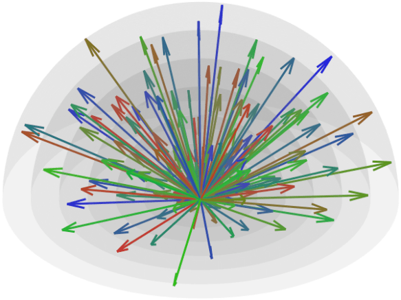
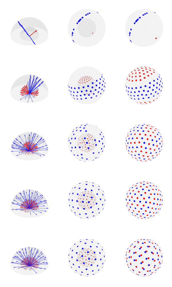
Basic plotting of the directions is available with the option –plot. When invoking from the shell, you can specify a file format for saving (e.g., pdf, eps, svg, png); four plots will be produced: with and without reprojecting all shells to unit sphere, and with the directions represented as arrows or as blobs.
./multishell.py --plot svg ...
If instead of a file format you provide the keyword interactive, it will open the plots in a window to allow interactive visualization, manipulation of the figure, and saving.
./multishell.py --plot interactive ...
Since antipodal points are included in the cost function, all directions can, for visualization purposes, be represented in only one hemisphere. However, that is only for display; the vectors themselves have equal likelihood of being in one hemisphere or another, thus covering the whole surface of the sphere.
Order of arguments and of operations
The order the arguments are provided is not relevant. If the same argument is repeated, it is the last one that counts. Inside the program, the operations happen in the following order:
- The options –new or –load are executed, thus either creating or loading a set of directions.
- If a file in a format that does not include b-values was loaded, or if a new set of directions was just created, the option –bvalues is parsed, thus defining the b-values for each shell.
- The option –reorder is executed if provided, thus optimally reordering the directions.
- The option –removeb0 is executed if provided, thus removing directions that have been assigned a b-value = 0.
- The option –addb0 is executed if provided, thus adding b-values = 0 and corresponding directions.
- The option –save is executed if provided, thus saving the set of directions to a file in the specified format.
- The option –plot is executed if provided, thus showing the directions (interactive mode) or saved to a file in the specified format (png, pdf, svg, eps, and various others supported by matplotlib).
Integration with your Python code
If you prefer not to use the function from the system shell and prefer instead to call it from your Python code, you can do that too. Place the file multishell.py where you can import it, then call the functions as needed. A simple example is:
import multishell as ms
import numpy as np

# Number of directions
K = 120

# Number of shells
S = 3

# b-values of each shell
blist = [1000, 2000, 3000]

# Distribute the number of directions across shells
Ks = ms.directions_per_shell(K, S, 'quadratically')

# Simultaneous optimization of all directions
vectors, shells = ms.simultaneous_optimization(Ks, alpha=0.75, maxiter=100)

# Optimally reorder the directions
vectors, shells, idx = ms.optimal_reordering(vectors, shells)

# b-values for each corresponding direction
bvalues = np.array(blist)[shells[:,0]][:,None]

# Save in FSL format
fileprefix = 'mydirs'
ms.write_fsl(fileprefix, vectors, bvalues)

# Plot
ms.plot_directions(vectors, bvalues=bvalues, colorby='acquisition', style='quiver', reproject=False)
Why a new implementation?
Two helpful implementations provided by Caruyer are available. One is a webtool that allows up to 5 shells and up to 500 directions be downloaded after estimation via incremental optimization, but it doesn’t allow specification of the weighting parameter
References
The most important reference is the original paper by Caruyer and colleagues, and which should be cited in case you use this reimplementation in your research:
- Caruyer E, Lenglet C, Sapiro G, Deriche R. Design of multishell sampling schemes with uniform coverage in diffusion MRI. Magn Reson Med. 2013 Jun;69(6):1534-40. doi: 10.1002/mrm.24736. Epub 2013 Apr 26. PMID: 23625329; PMCID: PMC5381389.
Other relevant work cited above are:
- Conturo TE, McKinstry RC, Akbudak E, Robinson BH. Encoding of anisotropic diffusion with tetrahedral gradients: a general mathematical diffusion formalism and experimental results. Magn Reson Med. 1996 Mar;35(3):399-412. doi: 10.1002/mrm.1910350319. PMID: 8699953.
- Jones DK, Horsfield MA, Simmons A. Optimal strategies for measuring diffusion in anisotropic systems by magnetic resonance imaging. Magn Reson Med. 1999 Sep;42(3):515-25. PMID: 10467296.
- Sotiropoulos SN, Jbabdi S, Xu J, Andersson JL, Moeller S, Auerbach EJ, Glasser MF, Hernandez M, Sapiro G, Jenkinson M, Feinberg DA, Yacoub E, Lenglet C, Van Essen DC, Ugurbil K, Behrens TE; WU-Minn HCP Consortium. Advances in diffusion MRI acquisition and processing in the Human Connectome Project. Neuroimage. 2013 Oct 15;80:125-43. doi: 10.1016/j.neuroimage.2013.05.057. Epub 2013 May 20. PMID: 23702418; PMCID: PMC3720790.
- Tuch DS. Q-ball imaging. Magn Reson Med. 2004 Dec;52(6):1358-72. doi: 10.1002/mrm.20279. PMID: 15562495.
 be a
be a  matrix of random values with zero mean and variance
  . The density of the bulk spectrum of the singular values
  ,
,  ,
, 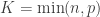 , of
, of  is:
is: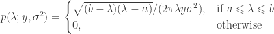
 at the origin if
  , where
  ,
,  , and
, and  (Bai, 1999). This is the Marčenko and Pastur (1967) distribution. The cumulative distribution function (cdf) can be obtained by integration, i.e.,
  .
.  or larger for a random matrix, we have the means to judge whether that
  of the sorted singular values. A different procedure needs be considered.
 versus the quantiles
  . Deviations from the identity line are evidence for excess variance not expected from random variables alone.
 is a matrix of observed variables,
  is a matrix of covariates (of no interest), and
  is a matrix of the same size as
  to compute the statistic of interest, and call this statistic
  .
. , obtaining estimated parameters
  and estimated residuals
  .
. . This is done by pre-multiplying the residuals from the reduced model produced in the previous step,
  , then adding back the estimated nuisance effects, i.e.
  .
.
 to compute the statistic of interest. Call this statistic
  .
. under the null hypothesis of no association between
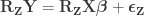
 is a permutation matrix (for the
  -th permutation,
  is the
  is the residual forming matrix; the superscript symbol
  represents a
 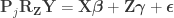 , implying that the permutations can actually be performed just by permuting the rows of the residual-forming matrix
  .
. .
. since
since  from an equivalent GLM written as
  .
.


 :
:
 :
:
 .
.


 cancels out, meaning that it is not necessary. Results are the same both ways.
 , growing uniformly and without gaps, and we see a tank that has a serial number
  . In that case, what would be the average value of the serial numbers of all
  , that is, the average of the first and last serial numbers.
 , our guess would be
  (that is, reorganizing the terms of the previous equation for
  ). Note that, for one sighting, this formula guarantees that
  , for ordered serial numbers
  . Clearly, we can’t use the same formula, because if
  (say, because we have seen many small serial numbers, but just a handful of larger ones),
  , the above formula gives invaluable insight: it shows that for such uniformly distributed data, approximately half of the tanks have serial number above
  (which is
  ) must be approximately the same as the (unknown) number of tanks above the highest serial number
  .
. . As it is based on all
  .
. . Then our best guess would be
  .
. , that is, the number of cases among those who travelled (
 ) divided by the total number of people who travelled (
 ) is expected to be approximately the same as the number of cases among those who stayed (
 ) divided by the total number of people who stayed (live) in the city (
 ).
). people travelling out, and
  staying in the city. The number of known international cases was at the time
  . Hence:
 cases
cases and
and  be two sets of variables over which CCA is computed. We find canonical coefficients
  and
and  ,
,  such that the canonical variables
  and
and  have maximal, diagonal correlation structure; this diagonal contains the ordered canonical correlations
  .
. and
and  be such correlations, which are termed canonical loadings or structure coefficients. Now compute the mean square for each of the columns of
  and
and  . These represent the variance extracted by the corresponding canonical variable. That is:
 :
: 
 :
: 
 , the usual coefficient of determination.
 and
and  and
and 

 of the surface representation, with vertex coordinates
 ![\mathbf{a}=[x_A \; y_A \; z_A]'](https://s0.wp.com/latex.php?latex=%5Cmathbf%7Ba%7D%3D%5Bx_A+%5C%3B+y_A+%5C%3B+z_A%5D%27&bg=ffffff&fg=333333&s=0&c=20201002) ,
, ![\mathbf{b}=[x_B \; y_B \; z_B]'](https://s0.wp.com/latex.php?latex=%5Cmathbf%7Bb%7D%3D%5Bx_B+%5C%3B+y_B+%5C%3B+z_B%5D%27&bg=ffffff&fg=333333&s=0&c=20201002) , and
, and ![\mathbf{c}=[x_C \; y_C \; z_C]'](https://s0.wp.com/latex.php?latex=%5Cmathbf%7Bc%7D%3D%5Bx_C+%5C%3B+y_C+%5C%3B+z_C%5D%27&bg=ffffff&fg=333333&s=0&c=20201002) , the area is
, the area is  , where
  ,
,  ,
,  represents the cross product, and the bars
  represent the vector norm. Even though such area per face (i.e., facewise) can be used in subsequent steps, most software packages can only deal with values assigned to each vertex (i.e., vertexwise). Conversion from facewise to vertexwise is achieved by assigning to each vertex one-third of the sum of the areas of all faces that meet at that vertex (

 in the white surface, and its corresponding face
  in the pial surface, define an oblique truncated triangular pyramid.
 ,
,  ,
,  and
and  represent its four vertices in terms of coordinates
 ![[x\;y\;z]'](https://s0.wp.com/latex.php?latex=%5Bx%5C%3By%5C%3Bz%5D%27&bg=ffffff&fg=333333&s=0&c=20201002) . Compute the volume as
. Compute the volume as  , where
  ,
,  ,
,  , the symbol
  represents the dot product, and the bars