Downsampling (decimating) a brain surface

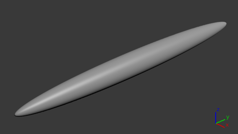
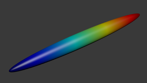
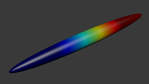
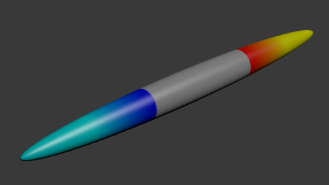
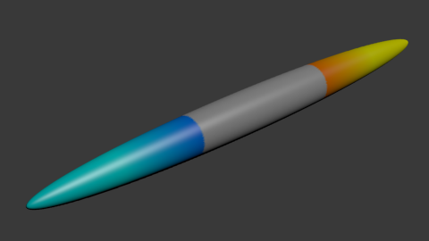
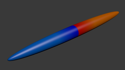
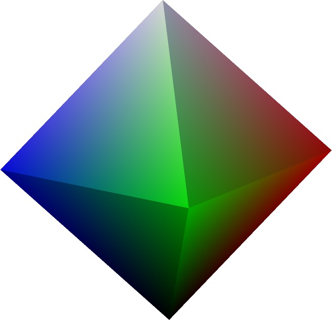
Downsampled average cortical surfaces at different iterations (n), with the respective number of vertices (V), edges (E) and faces (F).

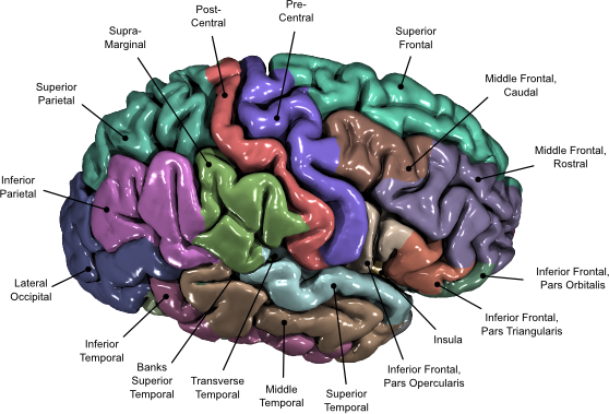
In the previous post, a method to display brain surfaces interactively in PDF documents was presented. While the method is already much more efficient than it was when it first appeared some years ago, the display of highly resolved meshes can be computationally intensive, and may make even the most enthusiastic readers give up even opening the file.

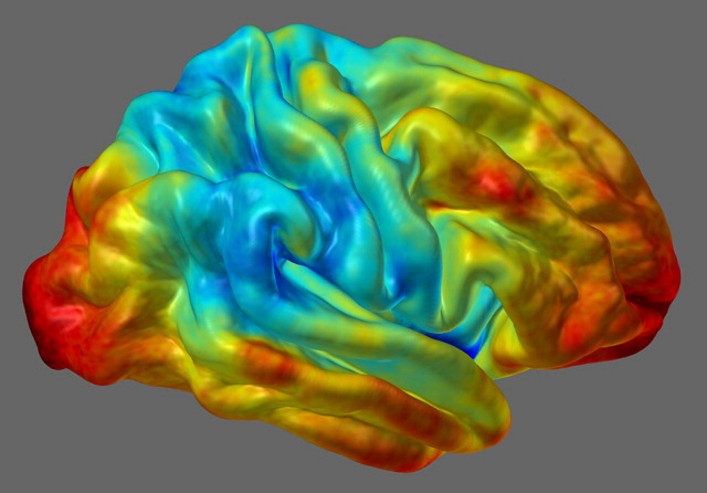
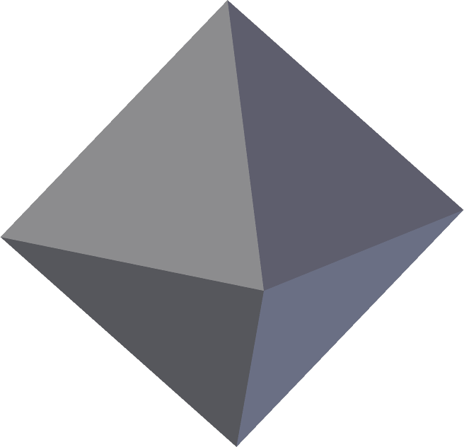
If the data being shown has low spatial frequency, an alternative way to display, which preserves generally the amount of information, is to decimate the mesh, downsampling it to a lower resolution. Although in theory this can be done in the native (subject-level) geometry through retessellation (i.e., interpolation of coordinates), the interest in downsampling usually is at the group level, in which case the subjects have all been interpolated to a common grid, which in general is a geodesic sphere produced by subdividing recursively an icosahedron (see this earlier post). If, at each iteration, the vertices and faces are added in a certain order (such as in FreeSurfer‘s fsaverage or in the one generated with the platonic command), downsampling is relatively straightforward, whatever is the type of data.

Vertexwise data

For vertexwise data, downsampling can be based on the fact that vertices are added (appended) in a certain order as the icosahedron is constructed:

  • Vertices 1-12 correspond to n = 0, i.e., no subdivision, or ico0.
  • Vertices 13-42 correspond to the vertices that, once added to the ico0, make it ico1 (first iteration of subdivision, n = 1).
  • Vertices 43-162 correspond to the vertices that, once added to ico1, make it ico2 (second iteration, n = 2).
  • Vertices 163-642, likewise, make ico3.
  • Vertices 643-2562 make ico4.
  • Vertices 2563-10242 make ico5.
  • Vertices 10243-40962 make ico6, etc.

Thus, if the data is vertexwise (also known as curvature, such as cortical thickness or curvature indices proper), the above information is sufficient to downsample the data: to reduce down to an ico3, for instance, all what one needs to do is to pick the vertices 1 through 642, ignoring 643 onwards.

Facewise data

Data stored at each face (triangle) generally correspond to areal quantities, that require mass conservation. For both fsaverage and platonic icosahedrons, the faces are added in a particular order such that, at each iteration of the subdivision, a given face index is replaced in situ for four other faces: one can simply collapse (via sum or average) the data of every four faces into a new one.

Surface geometry

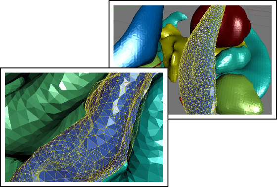
If the objective is to decimate the surface geometry, i.e., the mesh itself, as opposed to quantities assigned to vertices or faces, one can use similar steps:

  1. Select the vertices from the first up to the last vertex of the icosahedron in the level needed.
  2. Iteratively downsample the face indices by selecting first those that are formed by three vertices that were appended for the current iteration, then for those that have two vertices appended in the current iteration, then connecting the remaining three vertices to form a new, larger face.

Applications

Using downsampled data is useful not only to display meshes in PDF documents, but also, some analyses may not require a high resolution as the default mesh (ico7), particularly for processes that vary smoothly across the cortex, such as cortical thickness. Using a lower resolution mesh can be just as informative, while operating at a fraction of the computational cost.

A script

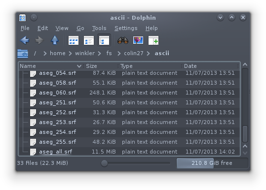
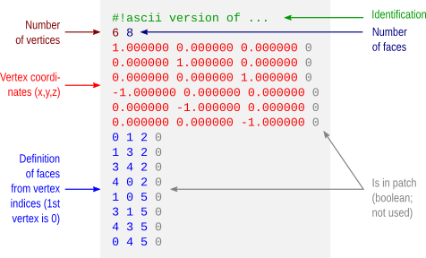
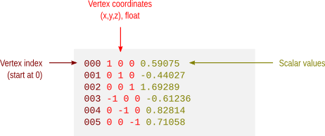
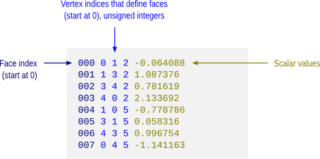
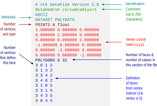
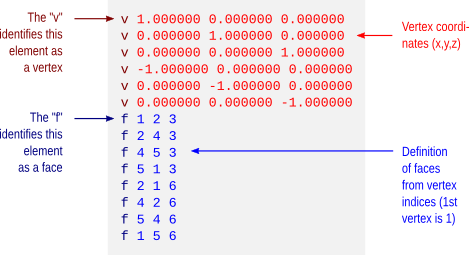
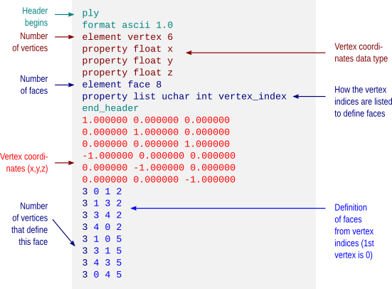
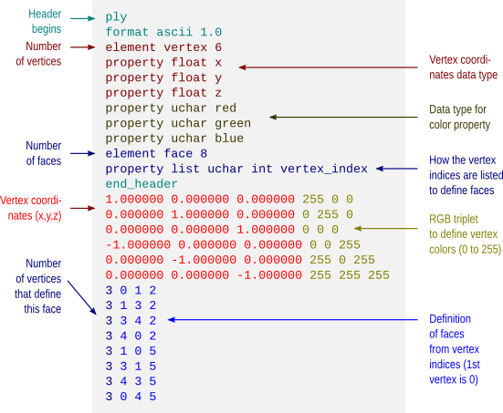
A script that does the tasks above using Matlab/Octave is here: icodown.m. It is also available as part of the areal package described here, which also satisfies all its dependencies. Input and output formats are described here.

Splitting the cortical surface into independent regions

FreeSurfer offers excellent visualisation capabilities with tksurfer and FreeView. However, there are endless other possibilities using various different computer graphics software. In previous posts, it was shown here in the blog how to generate cortical and subcortical surfaces that could be imported into these applications, as well as how to generate models with vertexwise and facewise colours, and even a description of common file formats. It was also previously shown how to arbitrarily change the colours of regions for use with FreeSurfer own tools. However, a method to allow rendering cortical regions with different colours in software such as Blender was missing. This is what this post is about.

The idea is simple: splitting the cortical surface into one mesh per parcellation allows each to be imported as an independent object, and so, it becomes straightforward to apply a different colour for each one. To split, the first step is to convert the FreeSurfer annotation file to a data-per-vertex file (*.dpv). This can be done with the command annot2dpv.

./annot2dpv lh.aparc.annot lh.aparc.annot.dpv

Before running, be sure that ${FREESURFER_HOME}/matlab is in the Octave/matlab, path. With the data-per-vertex file ready, do the splitting of the surface with splitsrf:

./splitsrf lh.white lh.aparc.annot.dpv lh.white_roi

This will create several files names as lh.white_roi*. Each corresponds to one piece of the cortex, in *.srf format. To convert to a format that can be read directly into computer graphics software, see the instructions here.

The annot2dpv and splitsrf are now included in the package for areal analysis, available here.

With the meshes imported, let your imagination and creativity fly. Once produced, labels can be added to the renderings using software such as Inkscape, to produce images as the one above, of the Desikan-Killiany atlas, which illustrates the paper Cortical Thickness or Gray Matter Volume: The Importance of Selecting the Phenotype for Imaging Genetics Studies.

Another method is also possible, without the need to split the cortex, but instead, painting the voxels. This can be done with the command replacedpx, also available from the package above. In this case each region index is replaced by its corresponding statistical value (or any other value), then maps are produced with the dpx2map, shown in an earlier blog post, here. This other method, however, requires that the label indices are known for each region, which in FreeSurfer depends on the rgb colors assigned to them. Moreover, the resulting maps don’t have as sharp and beautiful borders as when the surface is split into independent pieces.

Displaying vertexwise and facewise brain maps

In a previous post, a method to display FreeSurfer cortical regions in arbitrary colours was presented. Suppose that, instead, you would like to display the results from vertexwise or facewise analyses. For vertexwise, these can be shown using tksurfer or Freeview. The same does not apply, however, to facewise data, which, at the time of this writing, is not available in any neuroimaging software. In this article a tool to generate files with facewise or vertexwise data is provided, along with some simple examples.

The dpx2map tool

The tool to generate the maps is dpx2map (right-click to download, then make it executable). Call it without arguments to get usage information. This tool uses Octave as the backend, and it assumes that it is installed in its usual location (/usr/bin/octave). It is also possible to run it from inside Octave or Matlab using a slight variant, dpx2map.m (in which case, type help dpx2map for usage).

In either case, the commands srfread, dpxread and mtlwrite must be available. These are part of the areal package discussed here. And yes, dpx2map is now included in the latest release of the package too.

To use dpx2map, you need to specify a surface object that will provide the geometry on which the data colours will be overlaid, and the data itself. The surface should be in FreeSurfer format (*.asc or *.srf), and the data should be in FreeSurfer “curvature” format (*.asc, *.dpv) for vertexwise, or in facewise format (*.dpf). A description of these formats is available here.

It is possible to specify the data range that will be used when computing the scaling to make the colours, as well which range will be actually shown. It is also possible to split the scale so that a central part of it is omitted or shown in a colour outside the colourscale. This is useful to show thresholded positive and negative maps.

The output is saved either in Stanford Polygon (*.ply) for vertexwise, or in Wavefront Object (*.obj + *.mtl) for facewise data, and can be imported directly in many computer graphics software. All input and output files must be/are in their respective ascii versions, not binary. The command also outputs a image with the colourbar, in Portable Network Graphics format (*.png).

An example object

With a simple geometric shape as this it is much simpler to demonstrate how to generate the maps, than using a complicated object as the brain. The strategy for colouring remains the same. For the next examples, an ellipsoid was created using the platonic command. The command line used was:

platonic ellipsoid.obj ico sph 7 '[.25 0 0 0; 0 3 0 0; 0 0 .25 0; 0 0 0 1]'

This ellipsoid has maximum y-coordinate equal to 3, and a maximum x- and z-coordinates equal to 0.25. This file was converted from Wavefront *.obj to FreeSurfer ascii, and scalar fields simply describing the coordinates (x,y,z), were created with:

obj2srf ellipsoid.obj > ellipsoid.srf
srf2area ellipsoid.srf ellipsoid.dpv dpv
gawk '{print $1,$2,$3,$4,$2}' ellipsoid.dpv > ellipsoid-x.dpv
gawk '{print $1,$2,$3,$4,$3}' ellipsoid.dpv > ellipsoid-y.dpv
gawk '{print $1,$2,$3,$4,$4}' ellipsoid.dpv > ellipsoid-z.dpv

It is the ellipsoid-y.dpv that is used for the next examples.

Vertexwise examples

The examples below use the same surface (*.srf) and the same curvature, data-per-vertex file (*.dpv). The only differences are the way as the map is generated and presented, using different colour maps and different scaling. The jet colour map is the same available in Octave and Matlab. The coolhot5 is a custom colour map that will be made available, along with a few others, in another article to be posted soon.

Example A

In this example, defaults are used. The input files are specified, along with a prefix (exA) to be used to name the output files.

dpx2map ellipsoid-y.dpv ellipsoid.srf exA

Example B

In this example, the data between values -1.5 and 1.5 is coloured, and the remaining receive the colours of the extreme points (dark blue and dark red).

dpx2map ellipsoid-y.dpv ellipsoid.srf exB jet '[-1.5 1.5]'

Example C

In this example, the data between -2 and 2 is used to define the colours, with the values below/above receiving the extreme colours. However, the range between -1 and 1 is not shown or used for the colour scaling. This is because the dual option is set as true as well as the coption.

dpx2map ellipsoid-y.dpv ellipsoid.srf exC coolhot5 '[-2 2]' '[-1 1]' true '[.75 .75 .75]' true

Example D

This example is similar as above, except that the values between -1 and 1, despite not being shown, are used for the scaling of the colours. This is due to the coption being set as true.

dpx2map ellipsoid-y.dpv ellipsoid.srf exD coolhot5 '[-2 2]' '[-1 1]' true '[.75 .75 .75]' false

Example E

Here the data between -2 and 2 is used for scaling, but only the points between -1 and 1 are shown. This is because the option dual was set as false. The values below -1 or above 1 receive the same colours as these numbers, because the coption was configured as true. Note that because all points will receive some colour, it is not necessary to define the colourgap.

dpx2map ellipsoid-y.dpv ellipsoid.srf exE coolhot5 '[-2 2]' '[-1 1]' false '[]' true

Example F

This is similar as the previous example, except that the values between -1 and 1 receive a colour off of the colour map. This is because both dual and coption were set as false.

dpx2map ellipsoid-y.dpv ellipsoid.srf exF coolhot5 '[-2 2]' '[-1 1]' false '[.75 .75 .75]' false

Facewise data

The process to display facewise data is virtually identical. The only two differences are that (1) instead of supplying a *.dpv file, a *.dpf file is given to the script as input, and (2) the output isn’t a *.ply file, but instead a pair of files *.obj + *.mtl. Note that very few software can handle thousands of colours per object in the case of facewise data. Blender is recommended over most commercial products specially for this reason (and of course, it is free, as in freedom).

Download

The dpx2map is available here, and it is also included in the areal package, described here, where all its dependencies are satisfied. You must have Octave (free) or Matlab available to use this tool.

How to cite

If you use dpx2map for your scientific research, please, remember to mention the brainder.org website in your paper.

Update: Display in PDF documents

3D models as these, with vertexwise colours, can be shown in interactive PDF documents. Details here.

Merging multiple surfaces

Say you have a number of meshes in FreeSurfer ascii format (with extension *.asc or *.srf), one brain structure per file. However, for later processing or to import in some computer graphics software, you would like to have these multiple meshes all in a single file. This post provides a small script to accomplish this: mergesrf.

To use it, right click and save the file above, make it executable and, ideally, put it in a place where it can be found (or add its location to the environmental variable ${PATH}. Then run something as:

mergesrf file1.srf file2.srf fileN.srf mergedfile.srf

In this example, the output file is saved as mergedfile.srf. Another example is to convert all subcortical structures into just one large object, after aseg2srf as described here. To convert all, just change the current directory to ${SUBJECTS_DIR}//ascii, then run:

mergesrf * aseg_all.srf

A list with the input files and the output at the end is shown below:

The script uses Octave, which can be downloaded freely. The same script, with a small modification, can also run from inside matlab. This other version can be downloaded here: mergesrf.m

Requirements

In addition to Octave (or matlab), the script also requires functions to read and write surface files, which are available from the areal package (described here and downloadable here).

Brain meshes available

A set of 3D brain meshes produced with FreeSurfer and individually partitioned into separate files following the atlases of Desikan-Killiany, Destrieux et al., and Desikan-Killiany-Tourville (DKT), is now available for download here. Surfaces for subcortical structures are also available.

These meshes are meant to be used to help with scientific visualisation and/or artistic rendering in computer graphics software, most prominently Blender, but also in any other application that can import files in Wavefront (*.obj) or Stanford Polygon (*.ply) formats. The released files are under a Creative Commons license. See the download page for details.

Braindering with ASCII files

Binary file formats are faster to read and occupy less space for storage. However, when developing tools or when analysing data using non-standard methods, ascii files are easier to treat, and allow certain errors to be spotted immediately. Working with ascii files offer a number of advantages in these circumstances: the content of the files are human readable, meaning that there is no need for any special program other than perhaps a simple text editor, and can be manipulated easily with tools as sed or awk. It should be noted though, that while binary files require attention with respect to endianess and need some metadata to be correctly read, ascii need proper attention to end-of-line characters, that vary according to the operating system.

In articles to be posted soon I hope to share some tools to analyse and visualise brain imaging data. To use these tools, the files must be in ascii format. Each of these formats is discussed below and an example is given for a simple octahedron.

FreeSurfer surface (*.asc | suggested: *.srf)

FreeSurfer natively saves its surface files in binary form. The command mris_convert allows conversion to ascii format. The file extension is *.asc. This extension, however, is ambiguous with the curvature format (see below), reason for which a recommendation is to rename from *.asc to *.srf immediately after conversion.

The *.asc/*.srf format has a structure as described below. This format does not allow storing normals, colors, materials, multiple objects or textures. Just simple geometry.

FreeSurfer curvature (*.asc | suggested: *.dpv)

A curvature file contains a scalar value assigned to each vertex. This file format does not store the geometry of the surface and, in binary form, a curvature file simply contains one scalar per vertex. In ascii format, the vertex coordinates are also saved, but not how these vertices relate to define faces and the overall geometry.

Like with the FreeSurfer surface files, curvature files in ascii format also have the extension *.asc. To avoid confusion, it is suggested to rename from *.asc to *.dpv (data-per-vertex) immediately after conversion.

Facewise data (*.dpf)

This is not a native format from FreeSurfer, but a modification over the ascii curvature file described above. The file stores a scalar value per face, i.e. data-per-face (dpf) and, instead of saving vertex coordinates as with the *.dpv files, here the vertex indices that define the faces are saved. It is done like so because if both *.dpv and *.dpf files are present for a given geometric object, the object can be reconstructed with very little manipulation using simply awk. Currently there is no binary equivalent format.

VTK polygonal data (*.vtk)

A number of file formats have been developed over the years for use with the Visualization Toolkit (vtk). Some of these formats are now considered as “legacy” and are being phased out in favour of xml formats. Despite this, they are still used by a number of applications, such as fsl/first. The octahedron above in vtk polygonal data (polydata) format would have a structure as depicted below.

Wavefront Object (*.obj)

Wavefront Object files have a very simple structure, yet are powerful to allow definition of textures, normals and different materials. The format is supported by a variety of different graphic applications. The octahedron above would have a file structure as shown below.

The example does not show colors. However, it is possible to assign a material to each face, and materials contain their own color. These materials are typically stored in a separate file, a Materials Library, with extension *.mtl. An example for the same octahedron, both the object file and its associated materials library, is here: octa-color.obj and octa-color.mtl.


Many computer graphics software, however, limit the number of colors per object to a relatively small number, as 16 or 32. Blender, however, allows 32767 colors per object, a comfortable space for visualization of complex images, such as brain maps.

Stanford Polygon (*.ply)

The Stanford Polygon file allows not only the geometry to be stored, but also allow colours, transparency, confidence intervals and other properties to be assigned at each vertex. Again, the octahedron would have a file structure as:


This format also allows color attributes to be assigned to each vertex, as shown below.


The resulting object would then look like:

Batch conversion

Conversion between FreeSurfer formats can be done using mris_convert. A script to batch convert all FreeSurfer surface and curvature files from binary format to ascii is available here: subj2ascii. Before running, make sure FreeSurfer is correctly configured, that the variable SUBJECTS_DIR has been correctly set, and that you have writing permissions to this directory. Execute the script with no arguments to get usage information. The outputs (*.srf and *.dpv) are saved in a directory called ascii inside the directory of the subject. For many subjects, use a for-loop in the shell.

For more information

  • A description of the FreeSurfer file formats is available here.
  • A description of the different vtk (legacy and current) is available here.
  • Specification of the Wavefront obj format is here. Material library files are described here.
  • A description of the Stanford ply format is here.

Update — 28.May.2012: A script to convert from FreeSurfer .asc/.srf to .obj is here.
Update — 26.Jul.2013: This post was just updated to include examples of color formats.

Quickly inspect FreeSurfer cortical surfaces

To quickly inspect the surface reconstruction and parcellations produced by the cortical stream of FreeSurfer, rather than laboriously open each hemisphere at a time in tksurfer, an easier solution is to run a script that captures images, organise and present them all in a single html page that can be seen in any browser.

Before you start

Before you start, make sure you have:

  • FreeSurfer, any version released in the last 2 years. The procedure has been tested up to version 5.1.0.
  • ImageMagick, any recent version. For most Linux, ImageMagick can be installed directly from the distro’s repository. For Mac, it can be obtained with MacPorts or Fink.
  • The scripts takeshots, makehtml, shots_tksurfer.tcl, and shots_tkmedit.tcl. Put all these scripts into the same directory and make takeshots and makehtml executable.

Capturing the images

  1. Make sure recon-all finished for all your subjects. If there are no results, obviously there won’t be anything to inspect.
  2. Make sure the variable SUBJECTS_DIR is correctly set, pointing to the directory that contains the subjects, and that you have writing permissions to this directory.
  3. Prepare a text file containing a list of subjects, one per line, like this:
    subj001
    subj002
    ...
    subjNN
  4. Run the takeshots script. A typical usage is like this:
    ./takeshots -l listsubj.txt -m pial -m inflated -p aparc
    The options are:
    -l: List of subjects.
    -s: Additional subjects not in the list.
    -m: Surfaces to inspect (pial, inflated, white, sphere, etc).
    -p: Parcellations to inspect (aparc, aparc.a2005s, aparc.a2009s, etc).
    This script will create a subdirectory called ‘shots’ inside the directory of each subject, and will store a number of .tif files that are the different views of the cortical surfaces.
  5. Run the makehtml script. A typical usage is like this:
    ./makehtml -l listsubj.txt -m pial -m inflated -p aparc -d /path/to/html
    The options are identical to the previous command, with the addition of the option -d that lets you specify a directory where the html will be created. If this directory doesn’t exist, it will be created.

What you get

Open the file index.html in the directory specified in the previous step. There you’ll see all the surfaces of all the subjects, all in the same page, allowing you to quickly compare and have an idea of how good or bad they are. To see the name of the subject, hover the mouse on the corresponding image. Click on the image to see it larger. An example, using only pial and inflated surfaces, and the aparc parcellation, is here.