How do we measure thickness, area, and volume of the cerebral cortex?

Posted on 23.January.2018 by A. M. Winkler

There are various ways one could estimate morphometric parameters of the cortex, such as its thickness, area, and volume. For example, it is possible to use voxelwise partial volume effects using volume-based representations of the brain, such as in voxel-based morphometry (VBM), in which estimates per voxel become available. Volume-based representations also allow for estimates of thickness, as suggested, for example, by Hutton et al. (2004), or from a surface representation of the cortex, in which it can be measured as a form of distance between the mesh that represents the pia mater (the pial surface) and the mesh that represents the interface between gray and white matter (the white surface).

Here we focus on the surface-based representation as that offers advantages over volume-based representations (Van Essen et al., 1998). Software such as FreeSurfer uses magnetic resonance images to initially construct the white surface. Once that surface has been produced, a copy of it can be offset outwards until tissue contrast in the magnetic resonance image is maximal, which indicates the location of the pial surface. This procedure ensures that both white and pial surfaces have the same topology, with each face and each vertex of the white surface having their matching pair in the pial. This convenience facilitates the computations indicated below.

Cortical surface area

For a triangular face $ABC$ of the surface representation, with vertex coordinates $\mathbf{a}=[x_A \; y_A \; z_A]'$ , $\mathbf{b}=[x_B \; y_B \; z_B]'$ , and $\mathbf{c}=[x_C \; y_C \; z_C]'$ , the area is $|\mathbf{u} \times \mathbf{v}|/2$ , where $\mathbf{u} = \mathbf{a}-\mathbf{c}$ , $\mathbf{v} = \mathbf{b}-\mathbf{c}$ , $\times$ represents the cross product, and the bars $|\;|$ represent the vector norm. Even though such area per face (i.e., facewise) can be used in subsequent steps, most software packages can only deal with values assigned to each vertex (i.e., vertexwise). Conversion from facewise to vertexwise is achieved by assigning to each vertex one-third of the sum of the areas of all faces that meet at that vertex (Winkler et al., 2012).

Cortical thickness

The thickness at each vertex is computed as the average of two distances (Fischl and Dale, 2000; Greve and Fischl, 2018): the first is the distance from each white surface vertex to their corresponding closest point on the pial surface (not necessarily at a pial vertex); the second is the distance from the corresponding pial vertex to the closest point on the white surface (again, not necessarily at a vertex). Other methods are possible, however, see table below (adapted from Lerch and Evans, 2005):

Method	Reference
Distance solved using the Laplace’s equation.	Jones et al. (2000)
Distance between corresponding vertices.	MacDonald et al. (2000)
Distance to the nearest point in the other surface.	MacDonald et al. (2000)
Distance to the nearest point in the other surface, computed for both surfaces, then averaged.	Fischl and Dale (2000)
Distance along the normal.	MacDonald et al. (2000)
Distance along the iteratively computed normal.	Lerch and Evans (2005)

Cortical volume

Product method

If the area of either of these surfaces is known, or if the area of a mid-surface, i.e., the surface running half-distance between pial and white surfaces is known, an estimate of the volume can be obtained by multiplying, at each vertex, area by thickness. This procedure is still problematic in that it underestimates the volume of tissue that is external to the convexity of the surface, and overestimates volume that is internal to it; both cases are undesirable, and cannot be solved by merely resorting to using an intermediate surface as the mid-surface.

Figure 1: A diagram in two dimensions of the problem of measuring the cortical volume. If volume is computed using the product method (a), considerable amount of tissue is left unmeasured in the gyri, or measured repeatedly in sulci. The problem is minimised, but not solved, with the use of the mid-surface. In the analytic method (b), vertex coordinates are used to compute the volume of tissue between matching faces of white and pial surfaces, leaving no tissue under- or over-represented.

Analytic method

In Winkler et al. (2018) we propose a different approach to measure volume. Instead of computing the product of thickness and area, we note that any pair of matching faces can be used to define an irregular polyhedron, of which all six coordinates are known from the surface geometry. This polyhedron is an oblique truncated triangular pyramid, which can be perfectly divided into three irregular tetrahedra, which do not overlap, nor leave gaps.

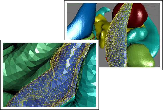
Figure 2: A 3D diagram with the proposed solution to measure the cortical volume. In the surface representation, the cortex is limited internally by the white and externally by the pial surface (a). These two surfaces have matching vertices that can be used to delineate an oblique truncated triangular pyramid (b) and (c). The six vertices of this pyramid can be used to define three tetrahedra, the volumes of which are computed analytically (d).

From the coordinates of the vertices of these tetrahedra, their volumes can be computed analytically, then added together, viz.:

For a given face $A_w B_w C_w$ in the white surface, and its corresponding face $A_p B_p C_p$ in the pial surface, define an oblique truncated triangular pyramid.
Split this truncated pyramid into three tetrahedra, defined as:
$\begin{array}{lcllllll} T_1 &=& (&A_w,&B_w,&C_w,&A_p&)\\ T_2 &=& (&A_p,&B_p,&C_p,&B_w&)\\ T_3 &=& (&A_p,&C_p,&C_w,&B_w&) \end{array}$
For each such tetrahedra, let $\mathbf{a}$ , $\mathbf{b}$ , $\mathbf{c}$ and $\mathbf{d}$ represent its four vertices in terms of coordinates $[x\;y\;z]'$ . Compute the volume as $|\mathbf{u}\cdot(\mathbf{v} \times \mathbf{w})|/6$ , where $\mathbf{u} = \mathbf{a}-\mathbf{d}$ , $\mathbf{v} = \mathbf{b}-\mathbf{d}$ , $\mathbf{w} = \mathbf{c}-\mathbf{d}$ , the symbol $\times$ represents the cross product, $\cdot$ represents the dot product, and the bars $|\;|$ represent the vector norm.

No error other than what is intrinsic to the placement of these surfaces is introduced. The resulting volume can be assigned to each vertex in a similar way as conversion from facewise area to vertexwise area. The above method is the default in FreeSurfer 6.0.0.

Is volume at all useful?

Given that volume of the cortex is, ultimately, determined by area and thickness, and these are known to be influenced in general by different factors (Panizzon et al, 2009; Winkler et al, 2010), why would anyone bother in even measuring volume? The answer is that not all factors that can affect the cortex will affect exclusively thickness or area. For example, an infectious process, or the development of a tumor, have potential to affect both. Volume is a way to assess the effects of such non-specific factors on the cortex. However, even in that case there are better alternatives available, namely, the non-parametric combination (NPC) of thickness and area. This use of NPC will be discussed in a future post here in the blog.

References

Fischl B, Dale AM. Measuring the thickness of the human cerebral cortex from magnetic resonance images. Proc Natl Acad Sci U S A. 2000 Sep 26;97(20):11050–5.
Greve DN, Fischl B. False positive rates in surface-based anatomical analysis. Neuroimage. 2018 Dec 26;171(1 May 2018):6–14.
Hutton C, De Vita E, Ashburner J, Deichmann R, Turner R. Voxel-based cortical thickness measurements in MRI. Neuroimage. 2008 May 1;40(4):1701–10.
Jones SE, Buchbinder BR, Aharon I. Three-dimensional mapping of cortical thickness using Laplace’s equation. Hum Brain Mapp. 2000 Sep;11(1):12–32.
Lerch JP, Evans AC. Cortical thickness analysis examined through power analysis and a population simulation. Neuroimage. 2005;24(1):163–73.
MacDonald D, Kabani NJ, Avis D, Evans AC. Automated 3-D extraction of inner and outer surfaces of cerebral cortex from MRI. Neuroimage. 2000 Sep;12(3):340–56.
Panizzon MS, Fennema-Notestine C, Eyler LT, Jernigan TL, Prom-Wormley E, Neale M, et al. Distinct genetic influences on cortical surface area and cortical thickness. Cereb Cortex. 2009 Nov;19(11):2728–35.
Van Essen DC, Drury HA, Joshi S, Miller MI. Functional and structural mapping of human cerebral cortex: solutions are in the surfaces. Proc Natl Acad Sci U S A. 1998 Feb 3;95(3):788–95.
Winkler AM, Kochunov P, Blangero J, Almasy L, Zilles K, Fox PT, et al. Cortical thickness or grey matter volume? The importance of selecting the phenotype for imaging genetics studies. Neuroimage. 2010 Nov 15;53(3):1135–46.
Winkler AM, Sabuncu MR, Yeo BTT, Fischl B, Greve DN, Kochunov P, et al. Measuring and comparing brain cortical surface area and other areal quantities. Neuroimage. 2012 Jul 15;61(4):1428–43.
Winkler AM, Greve DN, Bjuland KJ, Nichols TE, Sabuncu MR, Ha Berg AK, et al. Joint analysis of cortical area and thickness as a replacement for the analysis of the volume of the cerebral cortex. Cereb Cortex. 2018 Feb 1;28(2):738–49.

Downsampling (decimating) a brain surface

Posted on 31.May.2016 by A. M. Winkler

Downsampled average cortical surfaces at different iterations (n), with the respective number of vertices (V), edges (E) and faces (F).

In the previous post, a method to display brain surfaces interactively in PDF documents was presented. While the method is already much more efficient than it was when it first appeared some years ago, the display of highly resolved meshes can be computationally intensive, and may make even the most enthusiastic readers give up even opening the file.

If the data being shown has low spatial frequency, an alternative way to display, which preserves generally the amount of information, is to decimate the mesh, downsampling it to a lower resolution. Although in theory this can be done in the native (subject-level) geometry through retessellation (i.e., interpolation of coordinates), the interest in downsampling usually is at the group level, in which case the subjects have all been interpolated to a common grid, which in general is a geodesic sphere produced by subdividing recursively an icosahedron (see this earlier post). If, at each iteration, the vertices and faces are added in a certain order (such as in FreeSurfer‘s fsaverage or in the one generated with the platonic command), downsampling is relatively straightforward, whatever is the type of data.

Vertexwise data

For vertexwise data, downsampling can be based on the fact that vertices are added (appended) in a certain order as the icosahedron is constructed:

Vertices 1-12 correspond to n = 0, i.e., no subdivision, or ico0.
Vertices 13-42 correspond to the vertices that, once added to the ico0, make it ico1 (first iteration of subdivision, n = 1).
Vertices 43-162 correspond to the vertices that, once added to ico1, make it ico2 (second iteration, n = 2).
Vertices 163-642, likewise, make ico3.
Vertices 643-2562 make ico4.
Vertices 2563-10242 make ico5.
Vertices 10243-40962 make ico6, etc.

Thus, if the data is vertexwise (also known as curvature, such as cortical thickness or curvature indices proper), the above information is sufficient to downsample the data: to reduce down to an ico3, for instance, all what one needs to do is to pick the vertices 1 through 642, ignoring 643 onwards.

Facewise data

Data stored at each face (triangle) generally correspond to areal quantities, that require mass conservation. For both fsaverage and platonic icosahedrons, the faces are added in a particular order such that, at each iteration of the subdivision, a given face index is replaced in situ for four other faces: one can simply collapse (via sum or average) the data of every four faces into a new one.

Surface geometry

If the objective is to decimate the surface geometry, i.e., the mesh itself, as opposed to quantities assigned to vertices or faces, one can use similar steps:

Select the vertices from the first up to the last vertex of the icosahedron in the level needed.
Iteratively downsample the face indices by selecting first those that are formed by three vertices that were appended for the current iteration, then for those that have two vertices appended in the current iteration, then connecting the remaining three vertices to form a new, larger face.

Applications

Using downsampled data is useful not only to display meshes in PDF documents, but also, some analyses may not require a high resolution as the default mesh (ico7), particularly for processes that vary smoothly across the cortex, such as cortical thickness. Using a lower resolution mesh can be just as informative, while operating at a fraction of the computational cost.

A script

A script that does the tasks above using Matlab/Octave is here: icodown.m. It is also available as part of the areal package described here, which also satisfies all its dependencies. Input and output formats are described here.

Fast surface smoothing on a common grid

Posted on 30.November.2014 by A. M. Winkler

Smoothing scalar data on the surface of a high resolution sphere can be a slow process. If the filter is not truncated, the distances between all the vertices or barycentres of faces need to be calculated, in a very time consuming process. If the filter is truncated, the process can be faster, but with resolutions typically used in brain imaging, it can still be very slow, a problem that is amplified if data from many subjects are analysed.

However, if the data for each subject have already been interpolated to a common grid, such as an icosahedron recursively subdivided multiple times (details here), then the distances do not need to be calculated repeatedly for each of them. Doing so just once suffices. Furthermore, the implementation of the filter itself can be made in such a way that the smoothing process can be performed as a single matrix multiplication.

Consider the smoothing defined in Lombardi, (2002), which we used in Winkler et al., (2012):

$\tilde{Q}_n = \dfrac{\sum_j Q_j K\left(g\left(\mathbf{x}_n,\mathbf{x}_j\right)\right)}{\sum_j K\left(g\left(\mathbf{x}_n,\mathbf{x}_j\right)\right)}$

where $\tilde{Q}_n$ is the smoothed quantity at the vertex or face $n$ , $Q_j$ is the quantity assigned to the $j$ -th vertex or face of a sphere containining $J$ vertices or faces, $g\left(\mathbf{x}_n,\mathbf{x}_j\right)$ is the geodesic distance between vertices or faces with coordinates $\mathbf{x}_n$ and $\mathbf{x}_j$ , and $K(g)$ is the Gaussian filter, defined as a function of the geodesic distance between points.

The above formula requires that all distances between the current vertex or face $n$ and the other points $j$ are calculated, and that this is repeated for each $n$ , in a time consuming process that needs to be repeated over again for every additional subject. If, however, the distances $g$ are known and organised into a distance matrix $\mathbf{G}$ , the filter can take the form of a matrix of the same size, $\mathbf{K}$ , with the values at each row scaled so as to add up to unity, and the same smoothing can proceed as a simple matrix multiplication:

$\mathbf{\tilde{Q}} = \mathbf{K}\mathbf{Q}$

If the grid is the same for all subjects, which is the typical case when comparisons across subjects are performed, $\mathbf{K}$ can be calculated just once, saved, and reused for each subject.

It should be noted, however, that although running faster, the method requires much more memory. For a filter of full-width at half-maximum (FWHM) $f$ , truncated at a distance $t \cdot f$ from the filter center, in a sphere of radius $r$ , the number of non-zero elements in $\mathbf{K}$ is approximately:

$\text{nnz} \approx \dfrac{J^2}{2} \left(1-\cos\left(t \cdot \dfrac{f}{r}\right)\right)$

whereas the total number of elements is $J^2$ . Even using sparse matrices, this may require a large amount of memory space. For practical purposes, a filter with width $f$ = 20 mm can be truncated at twice the width ( $t$ = 2), for application in a sphere with 100 mm made by 7 subdivisions of an icosahedron, still comfortably in a computer with 16GB of RAM. Wider filters may require more memory to run.

The script smoothdpx, part of the areal interpolation tools, available here, can be used to do both things, that is, smooth the data for any given subject, and also save the filter so that it can be reused with other subjects. To apply a previously saved filter, the rpncalc can be used. These commands require Octave or MATLAB, and if Octave is available, they can be executed directly from the command line.

Figures

The figures above represent facewise data on the surface of a sphere of 100 mm radius, made by recursive subdivision of a regular icosahedron 4 times, constructed with the platonic command (details here), shown without smoothing, and smoothed with filters with FWHM = 7, 14, 21, 28 and 35 mm.

References

Lombardi M. Interpolation and smoothing. Astron. Astrophys. 2002; 395(2), 733–745.
Winkler AM, Sabuncu MR, Yeo BT, Fischl B, Greve DN, Kochunov P, Nichols TE, Blangero J, Glahn DC. Measuring and comparing brain cortical surface area and other areal quantities. Neuroimage. 2012 Jul 16;61(4):1428-43.

Splitting the cortical surface into independent regions

Posted on 08.January.2014 by A. M. Winkler

FreeSurfer offers excellent visualisation capabilities with tksurfer and FreeView. However, there are endless other possibilities using various different computer graphics software. In previous posts, it was shown here in the blog how to generate cortical and subcortical surfaces that could be imported into these applications, as well as how to generate models with vertexwise and facewise colours, and even a description of common file formats. It was also previously shown how to arbitrarily change the colours of regions for use with FreeSurfer own tools. However, a method to allow rendering cortical regions with different colours in software such as Blender was missing. This is what this post is about.

The idea is simple: splitting the cortical surface into one mesh per parcellation allows each to be imported as an independent object, and so, it becomes straightforward to apply a different colour for each one. To split, the first step is to convert the FreeSurfer annotation file to a data-per-vertex file (*.dpv). This can be done with the command annot2dpv.

./annot2dpv lh.aparc.annot lh.aparc.annot.dpv

Before running, be sure that ${FREESURFER_HOME}/matlab is in the Octave/matlab, path. With the data-per-vertex file ready, do the splitting of the surface with splitsrf:

./splitsrf lh.white lh.aparc.annot.dpv lh.white_roi

This will create several files names as lh.white_roi*. Each corresponds to one piece of the cortex, in *.srf format. To convert to a format that can be read directly into computer graphics software, see the instructions here.

The annot2dpv and splitsrf are now included in the package for areal analysis, available here.

With the meshes imported, let your imagination and creativity fly. Once produced, labels can be added to the renderings using software such as Inkscape, to produce images as the one above, of the Desikan-Killiany atlas, which illustrates the paper Cortical Thickness or Gray Matter Volume: The Importance of Selecting the Phenotype for Imaging Genetics Studies.

Another method is also possible, without the need to split the cortex, but instead, painting the voxels. This can be done with the command replacedpx, also available from the package above. In this case each region index is replaced by its corresponding statistical value (or any other value), then maps are produced with the dpx2map, shown in an earlier blog post, here. This other method, however, requires that the label indices are known for each region, which in FreeSurfer depends on the rgb colors assigned to them. Moreover, the resulting maps don’t have as sharp and beautiful borders as when the surface is split into independent pieces.

Displaying vertexwise and facewise brain maps

Posted on 28.July.2013 by A. M. Winkler

In a previous post, a method to display FreeSurfer cortical regions in arbitrary colours was presented. Suppose that, instead, you would like to display the results from vertexwise or facewise analyses. For vertexwise, these can be shown using tksurfer or Freeview. The same does not apply, however, to facewise data, which, at the time of this writing, is not available in any neuroimaging software. In this article a tool to generate files with facewise or vertexwise data is provided, along with some simple examples.

The dpx2map tool

The tool to generate the maps is dpx2map (right-click to download, then make it executable). Call it without arguments to get usage information. This tool uses Octave as the backend, and it assumes that it is installed in its usual location (/usr/bin/octave). It is also possible to run it from inside Octave or Matlab using a slight variant, dpx2map.m (in which case, type help dpx2map for usage).

In either case, the commands srfread, dpxread and mtlwrite must be available. These are part of the areal package discussed here. And yes, dpx2map is now included in the latest release of the package too.

To use dpx2map, you need to specify a surface object that will provide the geometry on which the data colours will be overlaid, and the data itself. The surface should be in FreeSurfer format (*.asc or *.srf), and the data should be in FreeSurfer “curvature” format (*.asc, *.dpv) for vertexwise, or in facewise format (*.dpf). A description of these formats is available here.

It is possible to specify the data range that will be used when computing the scaling to make the colours, as well which range will be actually shown. It is also possible to split the scale so that a central part of it is omitted or shown in a colour outside the colourscale. This is useful to show thresholded positive and negative maps.

The output is saved either in Stanford Polygon (*.ply) for vertexwise, or in Wavefront Object (*.obj + *.mtl) for facewise data, and can be imported directly in many computer graphics software. All input and output files must be/are in their respective ascii versions, not binary. The command also outputs a image with the colourbar, in Portable Network Graphics format (*.png).

An example object

With a simple geometric shape as this it is much simpler to demonstrate how to generate the maps, than using a complicated object as the brain. The strategy for colouring remains the same. For the next examples, an ellipsoid was created using the platonic command. The command line used was:

platonic ellipsoid.obj ico sph 7 '[.25 0 0 0; 0 3 0 0; 0 0 .25 0; 0 0 0 1]'

This ellipsoid has maximum y-coordinate equal to 3, and a maximum x- and z-coordinates equal to 0.25. This file was converted from Wavefront *.obj to FreeSurfer ascii, and scalar fields simply describing the coordinates (x,y,z), were created with:

obj2srf ellipsoid.obj > ellipsoid.srf
srf2area ellipsoid.srf ellipsoid.dpv dpv
gawk '{print $1,$2,$3,$4,$2}' ellipsoid.dpv > ellipsoid-x.dpv
gawk '{print $1,$2,$3,$4,$3}' ellipsoid.dpv > ellipsoid-y.dpv
gawk '{print $1,$2,$3,$4,$4}' ellipsoid.dpv > ellipsoid-z.dpv

It is the ellipsoid-y.dpv that is used for the next examples.

Vertexwise examples

The examples below use the same surface (*.srf) and the same curvature, data-per-vertex file (*.dpv). The only differences are the way as the map is generated and presented, using different colour maps and different scaling. The jet colour map is the same available in Octave and Matlab. The coolhot5 is a custom colour map that will be made available, along with a few others, in another article to be posted soon.

Example A

In this example, defaults are used. The input files are specified, along with a prefix (exA) to be used to name the output files.

dpx2map ellipsoid-y.dpv ellipsoid.srf exA

Example B

In this example, the data between values -1.5 and 1.5 is coloured, and the remaining receive the colours of the extreme points (dark blue and dark red).

dpx2map ellipsoid-y.dpv ellipsoid.srf exB jet '[-1.5 1.5]'

Example C

In this example, the data between -2 and 2 is used to define the colours, with the values below/above receiving the extreme colours. However, the range between -1 and 1 is not shown or used for the colour scaling. This is because the dual option is set as true as well as the coption.

dpx2map ellipsoid-y.dpv ellipsoid.srf exC coolhot5 '[-2 2]' '[-1 1]' true '[.75 .75 .75]' true

Example D

This example is similar as above, except that the values between -1 and 1, despite not being shown, are used for the scaling of the colours. This is due to the coption being set as true.

dpx2map ellipsoid-y.dpv ellipsoid.srf exD coolhot5 '[-2 2]' '[-1 1]' true '[.75 .75 .75]' false

Example E

Here the data between -2 and 2 is used for scaling, but only the points between -1 and 1 are shown. This is because the option dual was set as false. The values below -1 or above 1 receive the same colours as these numbers, because the coption was configured as true. Note that because all points will receive some colour, it is not necessary to define the colourgap.

dpx2map ellipsoid-y.dpv ellipsoid.srf exE coolhot5 '[-2 2]' '[-1 1]' false '[]' true

Example F

This is similar as the previous example, except that the values between -1 and 1 receive a colour off of the colour map. This is because both dual and coption were set as false.

dpx2map ellipsoid-y.dpv ellipsoid.srf exF coolhot5 '[-2 2]' '[-1 1]' false '[.75 .75 .75]' false

Facewise data

The process to display facewise data is virtually identical. The only two differences are that (1) instead of supplying a *.dpv file, a *.dpf file is given to the script as input, and (2) the output isn’t a *.ply file, but instead a pair of files *.obj + *.mtl. Note that very few software can handle thousands of colours per object in the case of facewise data. Blender is recommended over most commercial products specially for this reason (and of course, it is free, as in freedom).

Download

The dpx2map is available here, and it is also included in the areal package, described here, where all its dependencies are satisfied. You must have Octave (free) or Matlab available to use this tool.

How to cite

If you use dpx2map for your scientific research, please, remember to mention the brainder.org website in your paper.

Update: Display in PDF documents

3D models as these, with vertexwise colours, can be shown in interactive PDF documents. Details here.

Merging multiple surfaces

Posted on 11.July.2013 by A. M. Winkler

Say you have a number of meshes in FreeSurfer ascii format (with extension *.asc or *.srf), one brain structure per file. However, for later processing or to import in some computer graphics software, you would like to have these multiple meshes all in a single file. This post provides a small script to accomplish this: mergesrf.

To use it, right click and save the file above, make it executable and, ideally, put it in a place where it can be found (or add its location to the environmental variable ${PATH}. Then run something as:

mergesrf file1.srf file2.srf fileN.srf mergedfile.srf

In this example, the output file is saved as mergedfile.srf. Another example is to convert all subcortical structures into just one large object, after aseg2srf as described here. To convert all, just change the current directory to ${SUBJECTS_DIR}//ascii, then run:

mergesrf * aseg_all.srf

A list with the input files and the output at the end is shown below:

The script uses Octave, which can be downloaded freely. The same script, with a small modification, can also run from inside matlab. This other version can be downloaded here: mergesrf.m

Requirements

In addition to Octave (or matlab), the script also requires functions to read and write surface files, which are available from the areal package (described here and downloadable here).

Brain meshes available

Posted on 11.March.2013 by A. M. Winkler

A set of 3D brain meshes produced with FreeSurfer and individually partitioned into separate files following the atlases of Desikan-Killiany, Destrieux et al., and Desikan-Killiany-Tourville (DKT), is now available for download here. Surfaces for subcortical structures are also available.

These meshes are meant to be used to help with scientific visualisation and/or artistic rendering in computer graphics software, most prominently Blender, but also in any other application that can import files in Wavefront (*.obj) or Stanford Polygon (*.ply) formats. The released files are under a Creative Commons license. See the download page for details.

Facewise brain cortical surface area: scripts now available

Posted on 02.June.2012 by A. M. Winkler

In the paper Measuring and comparing brain cortical surface area and other areal quantities (Neuroimage, 2012;61(4):1428-43, doi:10.1016/j.neuroimage.2012.03.026, pmid:22446492), we described the steps to perform pycnophylactic interpolation, i.e., mass-conservative interpolation, of brain surface area. The method is also valid for any other quantity that is also areal by nature.

The scripts to perform the steps we propose in the paper are now freely available for Octave and/or matlab. They can also be executed directly from the shell using Octave as the interpreter. In this case, multiple instances can be easily submitted to run in a cluster. Click here to dowload and for step-by-step instructions.

Importing FreeSurfer subcortical structures into Blender

Posted on 08.May.2012 by A. M. Winkler

In a previous article, a method to import cortical meshes from FreeSurfer into Blender and other CG applications was presented. Here it is complemented with a method to import the subcortical structures. These structures are segmented as part of FreeSurfer subcortical stream, and are stored in a volume-based representation. In order to import into Blender, first it is necessary to generate surfaces, then convert to Wavefront OBJ, and finally, do the import. Below is an example of how the output looks like.

An example of a subcortical meshes generated from FreeSurfer subcortical segmentations imported into Blender.

Generating the surfaces for subcortical structures

The surfaces can be generated using FreeSurfer’s own tools. The script aseg2srf automates the task. Suppose you would like to create meshes for all subcortical structures of the subjects named “capitu”, “bentinho” and “ezequiel”. Simply run:

aseg2srf -s "capitu bentinho ezequiel"

The outputs are saved in a directory called ascii, inside each subject’s directory. The script requires that FreeSurfer is installed and working properly, and that the environmental variable ${SUBJECTS_DIR} has been set to point to the location where the subjects are. It is also necessary to have writing permissions to this directory, so that the surfaces can be saved.

If there are many subjects, provide a list from a text file, with one subject per line:

aseg2srf -s list.txt

To make surfaces for just some structures, provide their label numbers with the -l option. For the hippocampus, for instance, the labels are 17 and 53 for left and right respectively:

aseg2srf -s "capitu bentinho ezequiel" -l "17 53"

The script has also a -d option, for debugging, which allows to keep temporary files used during the mesh generation.

List of labels

Below is a list of the label codes for the major structures. A more comprehensive list is in the aseg.stats file, inside the stats directory for each subject, or in the FreeSurferColorLUT.txt file (in the FreeSurfer directory).

Left lateral ventricle	4
Left inferior part of the lateral ventricle	5
Left cerebellum white matter	7
Left cerebellum cortex	8
Left thalamus	10
Left caudate	11
Left putamen	12
Left pallidum	13
Left hippocampus	17
Left amygdala	18
CSF	24
Left accumbens	26
Left ventral diencephalon	28
Left choroid plexus	31
Right lateral ventricle	43
Right inferior part of the lateral ventricle	44
Right cerebellum white matter	46
Right cerebellum cortex	47
Right thalamus	49
Right caudate	50
Right putamen	51
Right pallidum	52
Right hippocampus	53
Right amygdala	54
Right accumbens	58
Right ventral diencephalon	60
Right choroid plexus	63
Corpus callosum, posterior part	251
Corpus callosum, middle posterior part	252
Corpus callosum, central part	253
Corpus callosum, middle anterior part	254
Corpus callosum, anterior part	255
3rd ventricle	14
4th ventricle	15
5th ventricle (CSF sometimes found in the septum pellucidum)	72
Brain stem	16

Conversion to Wavefront OBJ

Once the meshes have been generated, the process of conversion into a format that can be read by CG software is the same as described previously here.

Download

The script is available here: aseg2srf.

Requirements

FreeSurfer must be installed and working properly. The environmental variable ${SUBJECTS_DIR} must point to the directory where the data for each subject is located. It is also assumed that recon-all has been run successfully.

Importing FreeSurfer cortical meshes into Blender

Posted on 08.May.2012 by A. M. Winkler

Computer graphics (CG) applications, such as Blender, Maya or 3D Studio, doesn’t come with filters that allow to directly import or export FreeSurfer meshes. To import brain surfaces to these applications, converting first to an intermediate file format solves the problem. Below is an example of a brain imported into Blender.

An example of a brain mesh from FreeSurfer imported into Blender after conversion to Wavefront OBJ.

The mris_convert, from FreeSurfer, allows conversion to stereolithography format (STL). However, not all CG applications read natively from STL files. Moreover, other formats, such as Wavefront OBJ and Stanford PLY have simpler structure — yet allowing features that will be discussed here in forthcoming articles.

Conversion from FreeSurfer to Wavefront OBJ

A simple procedure to convert a FreeSurfer surface to Wavefront OBJ (ASCII) is:

1) Use mris_convert to convert from FreeSurfer binary to ASCII:

mris_convert lh.pial lh.pial.asc

2) A suggestion is to rename the .asc file to .srf, to differentiate it from other files that also have .asc extension and have a different internal structure.

mv lh.pial.asc lh.pial.srf

3) Use the script srf2obj to convert from .srf to .asc:

srf2obj lh.pial.srf > lh.pial.obj

The symbol “>” is necessary so that the output from srf2obj is redirected to a new file.

Conversion from Wavefront OBJ to FreeSurfer

To convert back to FreeSurfer, a similar strategy is used.

1) Use the script obj2srf to generate new .srf files (here directly named as .asc, as expected by mris_convert)

obj2srf lh.pial.obj > lh.pial.asc

2) Use mris_convert:

mris_convert lh.pial.asc lh.pial

Download

Both scripts are available here: srf2obj and obj2srf. Right-click and save, then make them executable.

Requirements

The scripts use gawk as the interpreter, and expects to find it on its usual location (/bin/gawk). If in your system gawk is installed elsewhere, modify the first line accordingly.

If you don’t have gawk, you can get it from the repository of your Linux distribution. For Mac, gawk is available in MacPorts and Fink. Alternatively, you may replace gawk with awk itself, nawk, or any other awk implementation that works.