Interactive 3D brains in PDF documents

Posted on 10.May.2016 by A. M. Winkler

A screenshot from Acrobat Reader. The example file is here.

Would it not be helpful to be able to navigate through tri-dimensional, surface-based representations of the brain when reading a paper, without having to download separate datasets, or using external software? Since 2004, with the release of the version 1.6 of the Portable Document Format (PDF), this has been possible. However, the means to generate the file were not easily available until about 2008, when Intel released of a set of libraries and tools. This still did not help much to improve popularity, as in-document rendering of complex 3D models requires a lot of memory and processing, making its use difficult in practice at the time. The fact that Acrobat Reader was a lot bloated did not help much either.

Now, almost eight years later, things have become easier for users who want to open these documents. Newer versions of Acrobat are much lighter, and capabilities of ordinary computers have increased. Yet, it seems the interest on this kind of visualisation have faded. The objective of this post is to show that it is remarkably simple to have interactive 3D objects in PDF documents, which can be used in any document published online, including theses, presentations, and papers: journals as PNAS and Journal of Neuroscience are at the forefront in accepting interactive manuscripts.

Requirements

U3D Tools: Make sure you have the IDTFConverter utility, from the U3D tools, available on SourceForge as part of the MathGL library. A direct link to version 1.4.4 is here; an alternative link, of a repackaged version of the same, is here. Compiling instructions for Linux and Mac are in the “readme” file. There are some dependencies that must be satisfied, and are described in the documentation. If you decide not to install the U3D tools, but only compile them, make sure the path of the executable is both in the $PATH and in the $LD_LIBRARY_PATH. This can be done with:

cd /path/to/the/directory/of/IDTFConverter
export PATH=${PATH}:$(pwd)
export LD_LIBRARY_PATH=${LD_LIBRARY_PATH}:$(pwd)

The ply2idtf function: Make sure you have the latest version of the areal package, which contains the MATLAB/Octave function ply2idtf.m used below.
Certain LaTeX packages: The packages movie15 or media9, that allow embedding the 3D object into the PDF using LaTeX. Either will work. Below it is assumed the older, movie15 package, is used.

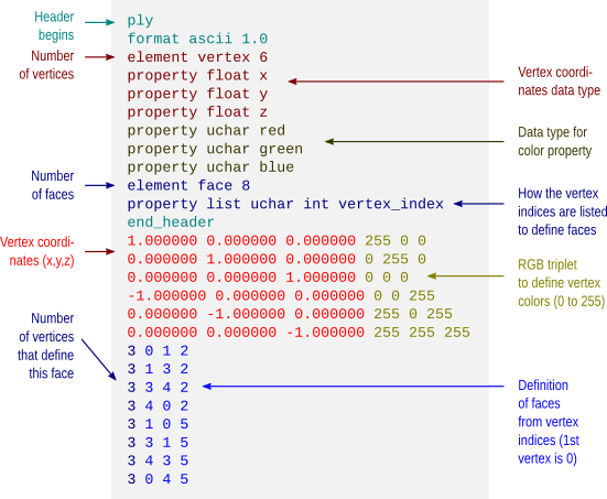
Step 1: Generate the PLY maps

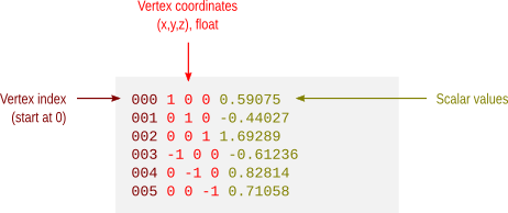
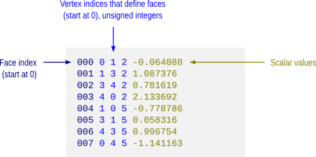
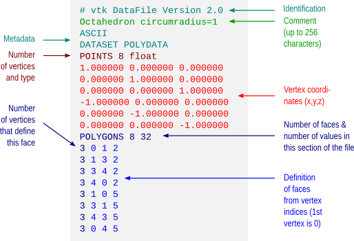
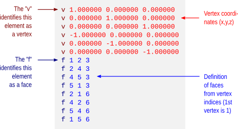
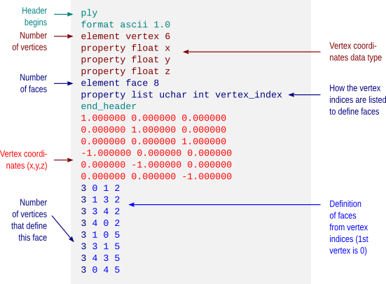
Once you have a map of vertexwise cortical data that needs to be shown, follow the instructions from this earlier blog post that explains how to generate Stanford PLY files to display colour-coded vertexwise data. These PLY files will be used below.

Step 2: Convert the PLY to IDTF files

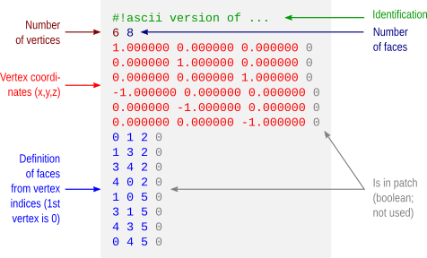
IDTF stands for Intermediate Data Text Format. As the name implies, it is a text, intermediate file, used as a step before the creation of the U3D files, the latter that are embedded into the PDF. Use the function ply2idtf for this:

ply2idtf(...
   {'lh.pial.thickness.avg.ply','LEFT', eye(4);...
    'rh.pial.thickness.avg.ply','RIGHT',eye(4)},...
    'thickness.idtf');

The first argument is a cell array with 3 columns, and as many rows as PLY files being added to the IDTF file. The first column contains the file name, the second the label (or node) that for that file, and the third an affine matrix that maps the coordinates from the PLY file to the world coordinate system of the (to be created) U3D. The second (last) argument to the command is the name of the output file.

Step 3: Convert the IDTF to U3D files

From a terminal window (not MATLAB or Octave), run:

IDTFConverter -input thickness.idtf -output thickness.u3d

Step 4: Configure default views

Here we use the older movie15 LaTeX package, and the same can be accomplished with the newer, media9 package. Various viewing options are configurable, all of which are described in the documentation. These options can be saved in a text file with extension .vws, and later supplied in the LaTeX document. An example is below.

VIEW=Both Hemispheres
  COO=0 -14 0,
  C2C=-0.75 0.20 0.65
  ROO=325
  AAC=30
  ROLL=-0.03
  BGCOLOR=.5 .5 .5
  RENDERMODE=Solid
  LIGHTS=CAD
  PART=LEFT
    VISIBLE=true
  END
  PART=RIGHT
    VISIBLE=true
  END
END
VIEW=Left Hemisphere
  COO=0 -14 0,
  C2C=-1 0 0
  ROO=325
  AAC=30
  ROLL=-0.03
  BGCOLOR=.5 .5 .5
  RENDERMODE=Solid
  LIGHTS=CAD
  PART=LEFT
    VISIBLE=true
  END
  PART=RIGHT
    VISIBLE=false
  END
END
VIEW=Right Hemisphere
  COO=0 -14 0,
  C2C=1 0 0
  ROO=325
  AAC=30
  ROLL=0.03
  BGCOLOR=.5 .5 .5
  RENDERMODE=Solid
  LIGHTS=CAD
  PART=LEFT
    VISIBLE=false
  END
  PART=RIGHT
    VISIBLE=true
  END
END

Step 5: Add the U3D to the LaTeX source

Interactive, 3D viewing is unfortunately not supported by most PDF readers. However, it is supported by the official Adobe Acrobat Reader since version 7.0, including the recent version DC. Thus, it is important to let the users/readers of the document know that they must open the file using a recent version of Acrobat. This can be done in the document itself, using a message placed with the option text of the \includemovie command of the movie15 package. A minimalistic LaTeX source is shown below (it can be downloaded here).

\documentclass{article}

% Relevant package:
\usepackage[3D]{movie15}

% pdfLaTeX and color links setup:
\usepackage{color}
\usepackage[pdftex]{hyperref}
\definecolor{colorlink}{rgb}{0, 0, .6}  % dark blue
\hypersetup{colorlinks=true,citecolor=colorlink,filecolor=colorlink,linkcolor=colorlink,urlcolor=colorlink}

\begin{document}
\title{Interactive 3D brains in PDF documents}
\author{}
\date{}
\maketitle

\begin{figure}[!h]
\begin{center}
\includemovie[
text=\fbox{\parbox[c][9cm][c]{9cm}{\centering {\footnotesize (Use \href{http://get.adobe.com/reader/}{Adobe Acrobat Reader 7.0+} \\to view the interactive content.)}}},
poster,label=Average,3Dviews2=pial.vws]{10cm}{10cm}{thickness.u3d}
\caption{An average 3D brain, showing colour-coded average thickness (for simplicity, colour scale not shown). Click to rotate. Right-click to for a menu with various options. Details at \href{http://brainder.org}{http://brainder.org}.}
\end{center}
\end{figure}

\end{document}

Step 6: Generate the PDF

For LaTeX, use pdfLaTeX as usual:

pdflatex document.tex

What you get

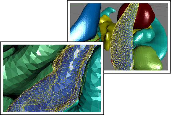
After generating the PDF, the result of this example is shown here (a screenshot is at the top). It is possible to rotate in any direction, zoom, pan, change views to predefined modes, and alternate between orthogonal and perspective projections. It’s also possible to change rendering modes (including transparency), and experiment with various lightning options.

In Acrobat Reader, by right-clicking, a menu with various useful options is presented. A toolbar (as shown in the top image) can also be enabled through the menu.

The same strategy works also with the Beamer class, such that interactive slides can be created and used in talks, and with XeTeX, allowing these with a richer variety of text fonts.

Brain meshes available

Posted on 11.March.2013 by A. M. Winkler

A set of 3D brain meshes produced with FreeSurfer and individually partitioned into separate files following the atlases of Desikan-Killiany, Destrieux et al., and Desikan-Killiany-Tourville (DKT), is now available for download here. Surfaces for subcortical structures are also available.

These meshes are meant to be used to help with scientific visualisation and/or artistic rendering in computer graphics software, most prominently Blender, but also in any other application that can import files in Wavefront (*.obj) or Stanford Polygon (*.ply) formats. The released files are under a Creative Commons license. See the download page for details.

Braindering with ASCII files

Posted on 25.September.2011 by A. M. Winkler

Binary file formats are faster to read and occupy less space for storage. However, when developing tools or when analysing data using non-standard methods, ascii files are easier to treat, and allow certain errors to be spotted immediately. Working with ascii files offer a number of advantages in these circumstances: the content of the files are human readable, meaning that there is no need for any special program other than perhaps a simple text editor, and can be manipulated easily with tools as sed or awk. It should be noted though, that while binary files require attention with respect to endianess and need some metadata to be correctly read, ascii need proper attention to end-of-line characters, that vary according to the operating system.

In articles to be posted soon I hope to share some tools to analyse and visualise brain imaging data. To use these tools, the files must be in ascii format. Each of these formats is discussed below and an example is given for a simple octahedron.

FreeSurfer surface (.asc | suggested: .srf)

FreeSurfer natively saves its surface files in binary form. The command mris_convert allows conversion to ascii format. The file extension is *.asc. This extension, however, is ambiguous with the curvature format (see below), reason for which a recommendation is to rename from *.asc to *.srf immediately after conversion.

The *.asc/*.srf format has a structure as described below. This format does not allow storing normals, colors, materials, multiple objects or textures. Just simple geometry.

FreeSurfer curvature (.asc | suggested: .dpv)

A curvature file contains a scalar value assigned to each vertex. This file format does not store the geometry of the surface and, in binary form, a curvature file simply contains one scalar per vertex. In ascii format, the vertex coordinates are also saved, but not how these vertices relate to define faces and the overall geometry.

Like with the FreeSurfer surface files, curvature files in ascii format also have the extension *.asc. To avoid confusion, it is suggested to rename from *.asc to *.dpv (data-per-vertex) immediately after conversion.

Facewise data (*.dpf)

This is not a native format from FreeSurfer, but a modification over the ascii curvature file described above. The file stores a scalar value per face, i.e. data-per-face (dpf) and, instead of saving vertex coordinates as with the *.dpv files, here the vertex indices that define the faces are saved. It is done like so because if both *.dpv and *.dpf files are present for a given geometric object, the object can be reconstructed with very little manipulation using simply awk. Currently there is no binary equivalent format.

VTK polygonal data (*.vtk)

A number of file formats have been developed over the years for use with the Visualization Toolkit (vtk). Some of these formats are now considered as “legacy” and are being phased out in favour of xml formats. Despite this, they are still used by a number of applications, such as fsl/first. The octahedron above in vtk polygonal data (polydata) format would have a structure as depicted below.

Wavefront Object (*.obj)

Wavefront Object files have a very simple structure, yet are powerful to allow definition of textures, normals and different materials. The format is supported by a variety of different graphic applications. The octahedron above would have a file structure as shown below.

The example does not show colors. However, it is possible to assign a material to each face, and materials contain their own color. These materials are typically stored in a separate file, a Materials Library, with extension *.mtl. An example for the same octahedron, both the object file and its associated materials library, is here: octa-color.obj and octa-color.mtl.

Many computer graphics software, however, limit the number of colors per object to a relatively small number, as 16 or 32. Blender, however, allows 32767 colors per object, a comfortable space for visualization of complex images, such as brain maps.

Stanford Polygon (*.ply)

The Stanford Polygon file allows not only the geometry to be stored, but also allow colours, transparency, confidence intervals and other properties to be assigned at each vertex. Again, the octahedron would have a file structure as:

This format also allows color attributes to be assigned to each vertex, as shown below.

The resulting object would then look like:

Batch conversion

Conversion between FreeSurfer formats can be done using mris_convert. A script to batch convert all FreeSurfer surface and curvature files from binary format to ascii is available here: subj2ascii. Before running, make sure FreeSurfer is correctly configured, that the variable SUBJECTS_DIR has been correctly set, and that you have writing permissions to this directory. Execute the script with no arguments to get usage information. The outputs (*.srf and *.dpv) are saved in a directory called ascii inside the directory of the subject. For many subjects, use a for-loop in the shell.

For more information

A description of the FreeSurfer file formats is available here.
A description of the different vtk (legacy and current) is available here.
Specification of the Wavefront obj format is here. Material library files are described here.
A description of the Stanford ply format is here.

Update — 28.May.2012: A script to convert from FreeSurfer .asc/.srf to .obj is here.
Update — 26.Jul.2013: This post was just updated to include examples of color formats.