Competition ranking and empirical distributions

Posted on 28.November.2012 by A. M. Winkler

Estimating the empirical cumulative distribution function (empirical cdf) from a set of observed values requires computing, for each value, how many of the other values are smaller or equal to it. In other words, let $X = \{x_1, x_2, \ldots , x_N\}$ be the observed values, then:

$F(x) = P(X \leqslant x) = \frac{1}{N} \sum_{n=1}^{N}I(x_n \leqslant x)$

where $F(x)$ is the empirical cdf, $P(X \leqslant x)$ is the probability of observing a value in $X$ that is smaller than or equal to $x$ , $I(\cdot)$ is a function that evaluates as 1 if the condition in the parenthesis is satisfied or 0 otherwise, and $N$ is the number of observations. This definition is straightforward and can be found in many statistical textbooks (see, e.g., Papoulis, 1991).

For continuous distributions, a p-value for a given $x \in X$ can be computed as $1-F(x)$ . For a discrete cdf, however, this trivial relationship does not hold. The reason is that, while for continuous distributions the probability $P(X = x) = 0$ , for discrete distributions (such as empirical distributions), $P(X = x) > 0$ whenever $x \in X$ . As we often want to assign a probability to one of the values that have been observed, the condition $x \in X$ always holds, and the simple relationship between the cdf and the p-value is lost. The solution, however, is still simple: a p-value can be obtained from the cdf as $1-F(x) + 1/N$ .

In the absence of repeated values (ties), the cdf can be obtained computationally by sorting the observed data in ascending order, i.e., $X_{s} = \{x_{(1)}, x_{(2)}, \ldots , x_{(N)}\}$ . Then $F(x)=(n_x)/N$ , where $(n_x)$ represents the ascending rank of $x$ . Likewise, the p-value can be obtaining by sorting the data in descending order, and using a similar formula, $P(X \geqslant x) = (\tilde{n}_x)/N$ , where $(\tilde{n}_x)$ represents the descending rank of $x$ .

Example 1: Consider the following sequence of 10 observed values, already sorted in ascending order:

$X=\{75, 76, 79, 80, 84, 85, 86, 88, 90, 94\}$

The corresponding ranks are simply 1, 2, 3, 4, 5, 6, 7, 8, 9, 10. Consequently, the cdf is:

$F(x|x\in X) = \{0.1, 0.2, 0.3, 0.4, 0.5, 0.6, 0.7, 0.8, 0.9, 1\}$

The p-values are computed by using the ranks in descending order, i.e., 10, 9, 8, 7, 6, 5, 4, 3, 2, 1, which yields:

$P(X \geqslant x | x \in X) = \{1, 0.9, 0.8, 0.7, 0.6, 0.5, 0.4, 0.3, 0.2, 0.1\}$

The problem with ties

Simple sorting, as above, is effective when there are no repeated values in the data. However, in the presence of ties, simple sorting that produces ordinal rankings yield incorrect results.

Example 2: Consider the following sequence of 10 observed values, in which ties are present:

$X = \{81, 81, 82, 83, 83, 83, 84, 85, 85, 85\}$

If the same computational strategy discussed above were used, the we would conclude that the p-value for $x=85$ would be either 0.1, 0.2 or 0.3, depending on which instance of the “85” we were to choose. The correct value, however, is 0.3 (only), since 3 out of 10 variables are equal or above 85. The solution to this problem is to replace the simple, ordinal ranking, for a modified version of the so called competition ranking.

The competition ranking

The competition ranking assigns the same rank to values that are identical. The standard competition ranking for the previous sequence is, in ascending order, 1, 1, 3, 4, 4, 4, 7, 8, 8, 8. In descending order, the ranks are 9, 9, 8, 5, 5, 5, 4, 1, 1, 1. Note that in this ranking, the ties receive the “best” possible rank. A slightly different approach consists in assigning the “worst” possible rank to the ties. This modified competition ranking applied the previous sequence gives, in ascending order, the ranks 2, 2, 3, 5, 5, 5, 7, 10, 10, 10, whereas in descending order, the ranks are 10, 10, 8, 7, 7, 7, 4, 3, 3, 3.

Competition ranking solves the problem with ties for both the empirical cdf and for the calculation of the p-values. In both cases, it is the modified version of the ranking that needs to be used, i.e., the ranking that assigns the worst rank to identical values. Still using the same sequence as example, the cdf is given by:

$F(x|x\in X) = \{0.2, 0.2, 0.3, 0.6, 0.6, 0.6, 0.7, 1, 1, 1\}$

and the p-values are given by:

$P(X \geqslant x | x \in X) = \{1, 1, 0.8, 0.7, 0.7, 0.7, 0.4, 0.3, 0.3, 0.3\}$

Note that, as in the case with no ties, the p-values cannot be computed simply as $1-F(x)$ from the cdf as it would for continuous distributions. The correct formula is $1-F(x)+(n_x)/N$ , with $(n_x)$ here representing the frequency of $x$ .

Uses

The cdf of a set of observed data is useful in many types of non-parametric inference, particularly those that use bootstrap, jack-knife, Monte Carlo, or permutation tests. Ties can be quite common when working with discrete data and discrete explanatory variables using any of these methods.

Competition ranking in MATLAB and Octave

A function that computes the competition ranks for Octave and/or MATLAB is available to download here: csort.m.

Once installed, type help csort to obtain usage information.

References

Papoulis A. Probability, Random Variables and Stochastic Processes. McGraw-Hill, New York, 3rd ed, 1991.

Automatic atlas queries in FSL

Posted on 30.July.2012 by A. M. Winkler

The fmrib Software Library (fsl) provides a tool to query whether regions belong or not to one of various atlases available. This well-known tool is called atlasquery, and it requires one region per image per run. To run for multiple separate regions on a single image image (e.g., a thresholded statistical map), a separate call to fsl‘s cluster command (not to be confused with the homonym cluster command that is part of the GraphViz package) is needed.

In order to automate this task, a small script called autoaq is available (UPDATE: the script is no longer supplied here; it has been incorporated into fsl). Usage information is provided by calling the command without arguments. This is the same script we posted recently to the fsl mailing list (here). Obviously, it does not run in Microsoft Windows. To use it, you need any recent Linux or Mac computer with fsl installed.

An example call is shown below:

./autoaq -i pvals.nii.gz -t 0.95 -o report.txt -a "JHU White-Matter Tractography Atlas"

The command will write temporary files to the directory from where it is called, hence it needs to be called from a directory to which the user has writing permissions. The atlas name can be any of the atlases available in fsl, currently being the ones listed below (note the quotes, ” “, that need to be provided when calling autoaq):

“Cerebellar Atlas in MNI152 space after normalization with FLIRT”
“Cerebellar Atlas in MNI152 space after normalization with FNIRT”
“Harvard-Oxford Cortical Structural Atlas”
“Harvard-Oxford Subcortical Structural Atlas”
“JHU ICBM-DTI-81 White-Matter Labels”
“JHU White-Matter Tractography Atlas”
“Juelich Histological Atlas”
“MNI Structural Atlas”
“Oxford Thalamic Connectivity Probability Atlas”
“Oxford-Imanova Striatal Connectivity Atlas 3 sub-regions”
“Oxford-Imanova Striatal Connectivity Atlas 7 sub-regions”
“Oxford-Imanova Striatal Structural Atlas”
“Talairach Daemon Labels”

The list can always be obtained through atlasquery --dumpatlases. Information about these atlases is available here.

The output is divided in three sections. In the first, a table containing the cluster indices, size and coordinates of the peaks and centres of mass is provided. In the second part, the structures to which the cluster peaks belong are presented, along with the associated probabilities. In the third part, probabilities for each cluster as a whole is presented. If the atlas is a binary label atlas, the number shown is in fact the overlap percentage between the cluster and the respective atlas label. If the atlas is probabilistic, the value is the mean probability in the overlapping region.

Version history:

03.Oct.2012: Update – Fixed issue with the md5 command under a different name in vanilla Mac.
25.Jan.2014: Update – Added options -u (to update/append a previous report) and -p to show peak coordinates instead of center of mass.
10.Dec.2014: The autoaq has been integrated into the freely available fmrib Software Library (fsl) and is no longer provided here. Hope you enjoy using it directly into fsl! :-)

Facewise brain cortical surface area: scripts now available

Posted on 02.June.2012 by A. M. Winkler

In the paper Measuring and comparing brain cortical surface area and other areal quantities (Neuroimage, 2012;61(4):1428-43, doi:10.1016/j.neuroimage.2012.03.026, pmid:22446492), we described the steps to perform pycnophylactic interpolation, i.e., mass-conservative interpolation, of brain surface area. The method is also valid for any other quantity that is also areal by nature.

The scripts to perform the steps we propose in the paper are now freely available for Octave and/or matlab. They can also be executed directly from the shell using Octave as the interpreter. In this case, multiple instances can be easily submitted to run in a cluster. Click here to dowload and for step-by-step instructions.

Retrospective motion correction for structural MRI

Posted on 17.May.2012 by A. M. Winkler

Good quality results can only be obtained with good quality images. To obtain images with good SNR and high resolution, long scan times are often necessary. However, with longer acquisition, the subjects are more likely to move. Rather than acquire a very long sequence, that often can last up to 40 minutes, the acquisition can be broken into many shorter scans, each with lower SNR. These are coregistered, effectively reducing the effect of undesired movement, and averaged, for increase of the SNR (Kochunov et al, 2006).

The last image in the second row is the average of all the other seven, after retrospective motion correction has been applied.

The results above are typical. Each pixel above corresponds to a true voxel, with no interpolation. Therefore, to see in more detail, simply download the image above and use an image viewer (e.g. gwenview or eog) to zoom.

The method is termed retrospective to discern it from prospective motion correction methods, such as those available for BOLD-sensitive EPI acquisitions (e.g. Siemens 3D PACE).

Since the images belong to the same subject and typically the movement is of only a few degrees or milimeters, the affine matrices for these corrections should have a diagonal with values very close to 1 and very close to zero off the diagonal. Here is one example:

0.999995    -0.00020007  -0.0030414    0.106906
0.000188555  0.999993    -0.00378601   0.100499
0.00304214   0.00378542   0.999988    -0.204133
0            0            0            1

As usual, the improvement in the SNR is given by a factor of $\sqrt{n}$ , where $n$ is the number of images averaged.

Download

A script to apply the method is available here: stereomc. Just download and make it executable. Call it without arguments to obtain usage information.

Requirements

FSL tools must be installed and properly configured.

Reference

Kochunov P, Lancaster JL, Glahn DC, Purdy D, Laird AR, Gao F, Fox P. Retrospective motion correction protocol for high-resolution anatomical MRI. Hum Brain Mapp. 2006 Dec;27(12):957-62.

Importing FreeSurfer subcortical structures into Blender

Posted on 08.May.2012 by A. M. Winkler

In a previous article, a method to import cortical meshes from FreeSurfer into Blender and other CG applications was presented. Here it is complemented with a method to import the subcortical structures. These structures are segmented as part of FreeSurfer subcortical stream, and are stored in a volume-based representation. In order to import into Blender, first it is necessary to generate surfaces, then convert to Wavefront OBJ, and finally, do the import. Below is an example of how the output looks like.

An example of a subcortical meshes generated from FreeSurfer subcortical segmentations imported into Blender.

Generating the surfaces for subcortical structures

The surfaces can be generated using FreeSurfer’s own tools. The script aseg2srf automates the task. Suppose you would like to create meshes for all subcortical structures of the subjects named “capitu”, “bentinho” and “ezequiel”. Simply run:

aseg2srf -s "capitu bentinho ezequiel"

The outputs are saved in a directory called ascii, inside each subject’s directory. The script requires that FreeSurfer is installed and working properly, and that the environmental variable ${SUBJECTS_DIR} has been set to point to the location where the subjects are. It is also necessary to have writing permissions to this directory, so that the surfaces can be saved.

If there are many subjects, provide a list from a text file, with one subject per line:

aseg2srf -s list.txt

To make surfaces for just some structures, provide their label numbers with the -l option. For the hippocampus, for instance, the labels are 17 and 53 for left and right respectively:

aseg2srf -s "capitu bentinho ezequiel" -l "17 53"

The script has also a -d option, for debugging, which allows to keep temporary files used during the mesh generation.

List of labels

Below is a list of the label codes for the major structures. A more comprehensive list is in the aseg.stats file, inside the stats directory for each subject, or in the FreeSurferColorLUT.txt file (in the FreeSurfer directory).

Left lateral ventricle	4
Left inferior part of the lateral ventricle	5
Left cerebellum white matter	7
Left cerebellum cortex	8
Left thalamus	10
Left caudate	11
Left putamen	12
Left pallidum	13
Left hippocampus	17
Left amygdala	18
CSF	24
Left accumbens	26
Left ventral diencephalon	28
Left choroid plexus	31
Right lateral ventricle	43
Right inferior part of the lateral ventricle	44
Right cerebellum white matter	46
Right cerebellum cortex	47
Right thalamus	49
Right caudate	50
Right putamen	51
Right pallidum	52
Right hippocampus	53
Right amygdala	54
Right accumbens	58
Right ventral diencephalon	60
Right choroid plexus	63
Corpus callosum, posterior part	251
Corpus callosum, middle posterior part	252
Corpus callosum, central part	253
Corpus callosum, middle anterior part	254
Corpus callosum, anterior part	255
3rd ventricle	14
4th ventricle	15
5th ventricle (CSF sometimes found in the septum pellucidum)	72
Brain stem	16

Conversion to Wavefront OBJ

Once the meshes have been generated, the process of conversion into a format that can be read by CG software is the same as described previously here.

Download

The script is available here: aseg2srf.

Requirements

FreeSurfer must be installed and working properly. The environmental variable ${SUBJECTS_DIR} must point to the directory where the data for each subject is located. It is also assumed that recon-all has been run successfully.

Importing FreeSurfer cortical meshes into Blender

Posted on 08.May.2012 by A. M. Winkler

Computer graphics (CG) applications, such as Blender, Maya or 3D Studio, doesn’t come with filters that allow to directly import or export FreeSurfer meshes. To import brain surfaces to these applications, converting first to an intermediate file format solves the problem. Below is an example of a brain imported into Blender.

An example of a brain mesh from FreeSurfer imported into Blender after conversion to Wavefront OBJ.

The mris_convert, from FreeSurfer, allows conversion to stereolithography format (STL). However, not all CG applications read natively from STL files. Moreover, other formats, such as Wavefront OBJ and Stanford PLY have simpler structure — yet allowing features that will be discussed here in forthcoming articles.

Conversion from FreeSurfer to Wavefront OBJ

A simple procedure to convert a FreeSurfer surface to Wavefront OBJ (ASCII) is:

1) Use mris_convert to convert from FreeSurfer binary to ASCII:

mris_convert lh.pial lh.pial.asc

2) A suggestion is to rename the .asc file to .srf, to differentiate it from other files that also have .asc extension and have a different internal structure.

mv lh.pial.asc lh.pial.srf

3) Use the script srf2obj to convert from .srf to .asc:

srf2obj lh.pial.srf > lh.pial.obj

The symbol “>” is necessary so that the output from srf2obj is redirected to a new file.

Conversion from Wavefront OBJ to FreeSurfer

To convert back to FreeSurfer, a similar strategy is used.

1) Use the script obj2srf to generate new .srf files (here directly named as .asc, as expected by mris_convert)

obj2srf lh.pial.obj > lh.pial.asc

2) Use mris_convert:

mris_convert lh.pial.asc lh.pial

Download

Both scripts are available here: srf2obj and obj2srf. Right-click and save, then make them executable.

Requirements

The scripts use gawk as the interpreter, and expects to find it on its usual location (/bin/gawk). If in your system gawk is installed elsewhere, modify the first line accordingly.

If you don’t have gawk, you can get it from the repository of your Linux distribution. For Mac, gawk is available in MacPorts and Fink. Alternatively, you may replace gawk with awk itself, nawk, or any other awk implementation that works.

Confidence intervals for Bernoulli trials

Posted on 21.April.2012 by A. M. Winkler

A Bernoulli trial is an experiment in which the outcome can be one of two mutually exclusive results, e.g. true/false, success/failure, heads/tails and so on. A number of methods are available to compute confidence intervals after many such trials have been performed. The most common have been discussed and reviewed by Brown et al. (2001), and are presented below. Consider $n$ trials, with $X$ successes and a significance level of $\alpha=0.05$ to obtain a 95% confidence interval. For each of the methods, the interval is shown graphically for $1 \leqslant n \leqslant 100$ and $1 \leqslant X \leqslant n$ .

Wald

This is the most common method, discussed in many textbooks, and probably the most problematic for small samples. It is based on a normal approximation to the binomial distribution, and it is often called “Wald interval” for it’s relationship with the Wald test. The interval is calculated as:

Lower bound: $L=p-k\sqrt{pq/n}$
Upper bound: $U=p+k\sqrt{pq/n}$

where $k = \Phi^{-1}\{1-\alpha/2\}$ , $\Phi^{-1}$ is the probit function, $p=X/n$ and $q=1-p$ .

Wald confidence interval.

Wilson

This interval appeared in Wilson (1927) and is defined as:

Lower bound: $L = \tilde{p} - (k/\tilde{n})\sqrt{npq+k^2/4}$
Upper bound: $U = \tilde{p} + (k/\tilde{n})\sqrt{npq+k^2/4}$

where $\tilde{p} = \tilde{X}/\tilde{n}$ , $\tilde{n}=n+k^2$ , $\tilde{X} = X+ k^2/2$ , and the remaining are as above. This is probably the most appropriate for the majority of situations.

Wilson confidence interval.

Agresti-Coull

This interval appeared in Agresti and Coull (1998) and shares many features with the Wilson interval. It is defined as:

Lower bound: $L = \tilde{p} - k\sqrt{\tilde{p}\tilde{q}/\tilde{n}}$
Upper bound: $U = \tilde{p} + k\sqrt{\tilde{p}\tilde{q}/\tilde{n}}$

where $\tilde{q}=1-\tilde{p}$ , and the remaining are as above.

Agresti-Coull confidence interval.

Jeffreys

This interval has a Bayesian motivation and uses the Jeffreys prior (Jeffreys, 1946). It seems to have been introduced by Brown et al. (2001). It is defined as:

Lower bound: $L = \mathcal{B}^{-1}\{\alpha/2,X+1/2,n-X+1/2\}$
Upper bound: $U = \mathcal{B}^{-1}\{1-\alpha/2,X+1/2,n-X+1/2\}$

where $\mathcal{B}^{-1}\{x,s_1,s_2\}$ is the inverse cdf of the beta distribution (not to be confused with the beta function), at the quantile $x$ , and with shape parameters $s_1$ and $s_2$ .

Jeffreys confidence interval.

Clopper-Pearson

This interval was proposed by Clopper and Pearson (1934) and is based on a binomial test, rather than on approximations, hence sometimes being called “exact”, although it is not “exact” in the common sense. It is considered overly conservative.

Lower bound: $L = \mathcal{B}^{-1}\{\alpha/2,X,n-X+1\}$
Upper bound: $U = \mathcal{B}^{-1}\{1-\alpha/2,X+1,n-X\}$

where $\mathcal{B}^{-1}\{x,s_1,s_2\}$ is the inverse cdf of the beta distribution as above.

Clopper-Pearson confidence interval.

Arc-Sine

This interval is based on the arc-sine variance-stabilising transformation. The interval is defined as:

Lower bound: $L = \sin\{\arcsin\{\sqrt{a}\} - k/(2\sqrt{n})\}^2$
Upper bound: $U = \sin\{\arcsin\{\sqrt{a}\} + k/(2\sqrt{n})\}^2$

where $a=\frac{X+3/8}{n+3/4}$ replaces what otherwise would be $p$ (Anscombe, 1948).

Arc-sine confidence interval.

Logit

This interval is based on the Wald interval for $\lambda = \ln\{\frac{X}{n-X}\}$ . It is defined as:

Lower bound: $L = e^{\lambda_L}/(1+e^{\lambda_L})$
Upper bound: $U = e^{\lambda_U}/(1+e^{\lambda_U})$

where $\lambda_L = \lambda - k\sqrt{\hat{V}}$ , $\lambda_U = \lambda + k\sqrt{\hat{V}}$ , and $\hat{V} = \frac{n}{X(n-X)}$ .

Logit confidence interval.

Anscombe

This interval was proposed by Anscombe (1956) and is based on the logit interval:

Lower bound: $L = e^{\lambda_L}/(1+e^{\lambda_L})$
Upper bound: $U = e^{\lambda_U}/(1+e^{\lambda_U})$

The difference is that $\lambda=\ln\{\frac{X+1/2}{n-X+1/2}\}$ and $\hat{V}=\frac{(n+1)(n+2)}{n(X+1)(n-X+1)}$ . The values for $\lambda_L$ and $\lambda_U$ are as above.

Anscombe’s confidence interval.

Octave/MATLAB implementation

A function that computes these intervals is available here: confint.m.

References

Agresti A and Coull BA. Approximate is better than “exact” for interval estimation of binomial proportions. The American Statistician. 1998; 52(2):119-126.
Anscombe FJ The transformation of Poisson, binomial and negative-binomial data. Biometrika. 1948; 35(3/4:246-254.
Anscombe FJ. On estimating binomial response relations. Biometrika. 1956; 43(3/4):461-464.
Brown LD, Cai TT, DasGupta A. Interval estimation for a binomial proportion. Statist Sci. 2001; 16(2):101-133.
Clopper CJ, Pearson ES. The use of confidence or fiducial limits illustrated in the case of the binomial. Biometrika. 1934; 26(4):404-413.
Jeffreys H. An invariant form for the prior probability in estimation problems. Proc. R. Soc. Lond. A. 1946; 186(1007):453-461.
Wilson EB. Probable inference, the law of succession, and statistical inference. J Am Stat Assoc. 1927; 22(158):209-21.

Braindering with ASCII files

Posted on 25.September.2011 by A. M. Winkler

Binary file formats are faster to read and occupy less space for storage. However, when developing tools or when analysing data using non-standard methods, ascii files are easier to treat, and allow certain errors to be spotted immediately. Working with ascii files offer a number of advantages in these circumstances: the content of the files are human readable, meaning that there is no need for any special program other than perhaps a simple text editor, and can be manipulated easily with tools as sed or awk. It should be noted though, that while binary files require attention with respect to endianess and need some metadata to be correctly read, ascii need proper attention to end-of-line characters, that vary according to the operating system.

In articles to be posted soon I hope to share some tools to analyse and visualise brain imaging data. To use these tools, the files must be in ascii format. Each of these formats is discussed below and an example is given for a simple octahedron.

FreeSurfer surface (.asc | suggested: .srf)

FreeSurfer natively saves its surface files in binary form. The command mris_convert allows conversion to ascii format. The file extension is *.asc. This extension, however, is ambiguous with the curvature format (see below), reason for which a recommendation is to rename from *.asc to *.srf immediately after conversion.

The *.asc/*.srf format has a structure as described below. This format does not allow storing normals, colors, materials, multiple objects or textures. Just simple geometry.

FreeSurfer curvature (.asc | suggested: .dpv)

A curvature file contains a scalar value assigned to each vertex. This file format does not store the geometry of the surface and, in binary form, a curvature file simply contains one scalar per vertex. In ascii format, the vertex coordinates are also saved, but not how these vertices relate to define faces and the overall geometry.

Like with the FreeSurfer surface files, curvature files in ascii format also have the extension *.asc. To avoid confusion, it is suggested to rename from *.asc to *.dpv (data-per-vertex) immediately after conversion.

Facewise data (*.dpf)

This is not a native format from FreeSurfer, but a modification over the ascii curvature file described above. The file stores a scalar value per face, i.e. data-per-face (dpf) and, instead of saving vertex coordinates as with the *.dpv files, here the vertex indices that define the faces are saved. It is done like so because if both *.dpv and *.dpf files are present for a given geometric object, the object can be reconstructed with very little manipulation using simply awk. Currently there is no binary equivalent format.

VTK polygonal data (*.vtk)

A number of file formats have been developed over the years for use with the Visualization Toolkit (vtk). Some of these formats are now considered as “legacy” and are being phased out in favour of xml formats. Despite this, they are still used by a number of applications, such as fsl/first. The octahedron above in vtk polygonal data (polydata) format would have a structure as depicted below.

Wavefront Object (*.obj)

Wavefront Object files have a very simple structure, yet are powerful to allow definition of textures, normals and different materials. The format is supported by a variety of different graphic applications. The octahedron above would have a file structure as shown below.

The example does not show colors. However, it is possible to assign a material to each face, and materials contain their own color. These materials are typically stored in a separate file, a Materials Library, with extension *.mtl. An example for the same octahedron, both the object file and its associated materials library, is here: octa-color.obj and octa-color.mtl.

Many computer graphics software, however, limit the number of colors per object to a relatively small number, as 16 or 32. Blender, however, allows 32767 colors per object, a comfortable space for visualization of complex images, such as brain maps.

Stanford Polygon (*.ply)

The Stanford Polygon file allows not only the geometry to be stored, but also allow colours, transparency, confidence intervals and other properties to be assigned at each vertex. Again, the octahedron would have a file structure as:

This format also allows color attributes to be assigned to each vertex, as shown below.

The resulting object would then look like:

Batch conversion

Conversion between FreeSurfer formats can be done using mris_convert. A script to batch convert all FreeSurfer surface and curvature files from binary format to ascii is available here: subj2ascii. Before running, make sure FreeSurfer is correctly configured, that the variable SUBJECTS_DIR has been correctly set, and that you have writing permissions to this directory. Execute the script with no arguments to get usage information. The outputs (*.srf and *.dpv) are saved in a directory called ascii inside the directory of the subject. For many subjects, use a for-loop in the shell.

For more information

A description of the FreeSurfer file formats is available here.
A description of the different vtk (legacy and current) is available here.
Specification of the Wavefront obj format is here. Material library files are described here.
A description of the Stanford ply format is here.

Update — 28.May.2012: A script to convert from FreeSurfer .asc/.srf to .obj is here.
Update — 26.Jul.2013: This post was just updated to include examples of color formats.

Quickly inspect FreeSurfer cortical surfaces

Posted on 10.September.2011 by A. M. Winkler

To quickly inspect the surface reconstruction and parcellations produced by the cortical stream of FreeSurfer, rather than laboriously open each hemisphere at a time in tksurfer, an easier solution is to run a script that captures images, organise and present them all in a single html page that can be seen in any browser.

Before you start

Before you start, make sure you have:

FreeSurfer, any version released in the last 2 years. The procedure has been tested up to version 5.1.0.
ImageMagick, any recent version. For most Linux, ImageMagick can be installed directly from the distro’s repository. For Mac, it can be obtained with MacPorts or Fink.
The scripts takeshots, makehtml, shots_tksurfer.tcl, and shots_tkmedit.tcl. Put all these scripts into the same directory and make takeshots and makehtml executable.

Capturing the images

Make sure recon-all finished for all your subjects. If there are no results, obviously there won’t be anything to inspect.
Make sure the variable SUBJECTS_DIR is correctly set, pointing to the directory that contains the subjects, and that you have writing permissions to this directory.
Prepare a text file containing a list of subjects, one per line, like this:
subj001 subj002 ... subjNN
Run the takeshots script. A typical usage is like this:
./takeshots -l listsubj.txt -m pial -m inflated -p aparc
The options are:
-l: List of subjects.
-s: Additional subjects not in the list.
-m: Surfaces to inspect (pial, inflated, white, sphere, etc).
-p: Parcellations to inspect (aparc, aparc.a2005s, aparc.a2009s, etc).
This script will create a subdirectory called ‘shots’ inside the directory of each subject, and will store a number of .tif files that are the different views of the cortical surfaces.
Run the makehtml script. A typical usage is like this:
./makehtml -l listsubj.txt -m pial -m inflated -p aparc -d /path/to/html
The options are identical to the previous command, with the addition of the option -d that lets you specify a directory where the html will be created. If this directory doesn’t exist, it will be created.

What you get

Open the file index.html in the directory specified in the previous step. There you’ll see all the surfaces of all the subjects, all in the same page, allowing you to quickly compare and have an idea of how good or bad they are. To see the name of the subject, hover the mouse on the corresponding image. Click on the image to see it larger. An example, using only pial and inflated surfaces, and the aparc parcellation, is here.

False Discovery Rate: Corrected & Adjusted P-values

Posted on 05.September.2011 by A. M. Winkler

Until mid-1990’s, control of the error rate under multiple testing was done, in general, using family-wise error rate (FWER). An example of this kind of correction is the Bonferroni correction. In an influential paper, Benjamini and Hochberg (1995) introduced the concept of false discovery rate (FDR) as a way to allow inference when many tests are being conducted. Differently than FWER, which controls the probability of committing a type I error for any of a family of tests, FDR allows the researcher to tolerate a certain number of tests to be incorrectly discovered. The word rate in the FDR is in fact a misnomer, as the FDR is the proportion of discoveries that are false among all discoveries, i.e., proportion of incorrect rejections among all rejections of the null hypothesis.

Benjamini and Hochberg’s FDR-controlling procedure

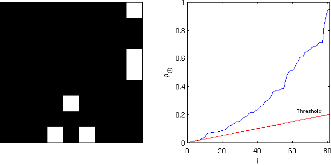
Consider testing $N$ hypotheses, $H_{1}, H_{2}, \ldots , H_{N}$ based on their respective p-values, $p_{1}, p_{2}, \ldots , p_{N}$ . Consider that a fraction $q$ of discoveries are allowed (tolerated) to be false. Sort the p-values in ascending order, $p_{(1)} \leq p_{(2)} \leq \ldots \leq p_{(N)}$ and denote $H_{(i)}$ the hypothesis corresponding to $p_{(i)}$ . Let $k$ be the largest $i$ for which $p_{(i)} \leq \frac{i}{N}\frac{q}{c(N)}$ . Then reject all $H_{(i)}$ , $i=1, 2, \ldots , k$ . The constant $c(N)$ is not in the original publication, and appeared in Benjamini and Yekutieli (2001) for cases in which independence cannot be ascertained. The possible choices for the constant are $c(N)=1$ or $c(N)=\sum_{i=1}^{N} 1/i$ . The second is valid in any situation, whereas the first is valid for most situations, particularly where there are no negative correlations among tests. The B&H procedure has found many applications across different fields, including neuroimaging, as introduced by Genovese et al. (2002).

FDR correction

The procedure described above effectively defines a single number, a threshold, that can be used to declare tests as significant or not at the level $q$ . One might, instead, be interested to know, for each original p-value, the minimum $q$ level in which they would still be rejected. To find this out, define $q_{(i)}=\frac{p_{(i)}N}{i}c(N)$ . This formulation, however, has problems, as discussed next.

FDR adjustment

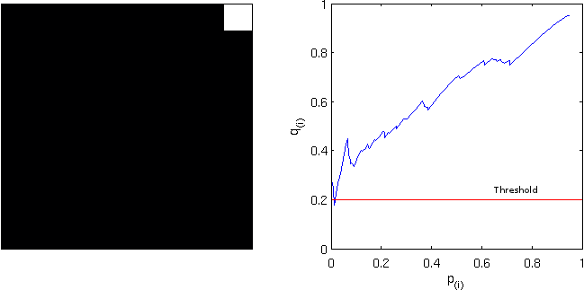
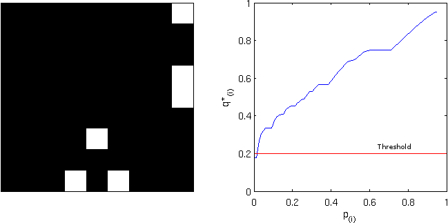
The problem with the FDR-correction is that $q_{(i)}$ is not a monotonic function of $p_{(i)}$ . This means that if someone uses any $q_{(i)}$ to threshold the set of FDR-corrected values, the result is not the same as would be obtained by applying sequentially the B&H procedure for all these corresponding $q$ levels.

To address this concern, Yekutieli and Benjamini (1999) introduced the FDR-adjustment, in which monotonicity is enforced, and which definition is compatible with the original FDR definition. Let $q*_{(i)}$ be the FDR-adjusted value for $p_{(i)}$ . It’s value is the smallest $q_{(k)}, k \geq i$ , where $q_{(k)}$ is the FDR-corrected as defined above. That’s just it!

Example

Consider the image below, on the left, a square of 9×9 pixels containing each some t-statistic with some sparse, low magnitude signal added. On the right are the corresponding p-values, ranging approximately between 0-1:

Statistical maps

Statistic and p-values

colorscale

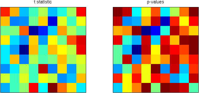
Using the B&H procedure to compute the threshold, with $q=0.20$ , and applying this threshold to the image rejects the null hypothesis in 6 pixels. On the right panel, the red line corresponds to the threshold. All p-values (in blue) below this line are declared significant.

FDR-threshold

FDR-threshold

Computing the FDR-corrected values at each pixel, and thresholding at the same $q=0.20$ , however, does not produce the same results, and just 1 pixel is declared significant. Although conservative, the “correction” is far from the nominal false discovery rate and is not appropriate. Note on the right panel the lack of monotonicity.

FDR-corrected

FDR-corrected

Computing instead the FDR-adjusted values, and thresholding again at $q=0.20$ produces the same results as with the simpler FDR-threshold. The adjustment is, thus, more “correct” than the “corrected”. Observe, on the right panel, the monotonicity enforced.

FDR-adjusted

FDR-adjusted

Implementation

An implementation of the three styles of FDR for Octave/MATLAB is available here: fdr.m
SPM users will find a similar feature in the function spm_P_FDR.m.