fdr correction

Until mid-1990’s, control of the error rate under multiple testing was done, in general, using family-wise error rate (FWER). An example of this kind of correction is the Bonferroni correction. In an influential paper, Benjamini and Hochberg (1995) introduced the concept of false discovery rate (FDR) as a way to allow inference when many tests are being conducted. Differently than FWER, which controls the probability of committing a type I error for any of a family of tests, FDR allows the researcher to tolerate a certain number of tests to be incorrectly discovered. The word rate in the FDR is in fact a misnomer, as the FDR is the proportion of discoveries that are false among all discoveries, i.e., proportion of incorrect rejections among all rejections of the null hypothesis.

Benjamini and Hochberg’s FDR-controlling procedure

Consider testing $N$ hypotheses, $H_{1}, H_{2}, \ldots , H_{N}$ based on their respective p-values, $p_{1}, p_{2}, \ldots , p_{N}$ . Consider that a fraction $q$ of discoveries are allowed (tolerated) to be false. Sort the p-values in ascending order, $p_{(1)} \leq p_{(2)} \leq \ldots \leq p_{(N)}$ and denote $H_{(i)}$ the hypothesis corresponding to $p_{(i)}$ . Let $k$ be the largest $i$ for which $p_{(i)} \leq \frac{i}{N}\frac{q}{c(N)}$ . Then reject all $H_{(i)}$ , $i=1, 2, \ldots , k$ . The constant $c(N)$ is not in the original publication, and appeared in Benjamini and Yekutieli (2001) for cases in which independence cannot be ascertained. The possible choices for the constant are $c(N)=1$ or $c(N)=\sum_{i=1}^{N} 1/i$ . The second is valid in any situation, whereas the first is valid for most situations, particularly where there are no negative correlations among tests. The B&H procedure has found many applications across different fields, including neuroimaging, as introduced by Genovese et al. (2002).

The procedure described above effectively defines a single number, a threshold, that can be used to declare tests as significant or not at the level $q$ . One might, instead, be interested to know, for each original p-value, the minimum $q$ level in which they would still be rejected. To find this out, define $q_{(i)}=\frac{p_{(i)}N}{i}c(N)$ . This formulation, however, has problems, as discussed next.

FDR adjustment

The problem with the FDR-correction is that $q_{(i)}$ is not a monotonic function of $p_{(i)}$ . This means that if someone uses any $q_{(i)}$ to threshold the set of FDR-corrected values, the result is not the same as would be obtained by applying sequentially the B&H procedure for all these corresponding $q$ levels.

To address this concern, Yekutieli and Benjamini (1999) introduced the FDR-adjustment, in which monotonicity is enforced, and which definition is compatible with the original FDR definition. Let $q*_{(i)}$ be the FDR-adjusted value for $p_{(i)}$ . It’s value is the smallest $q_{(k)}, k \geq i$ , where $q_{(k)}$ is the FDR-corrected as defined above. That’s just it!

Example

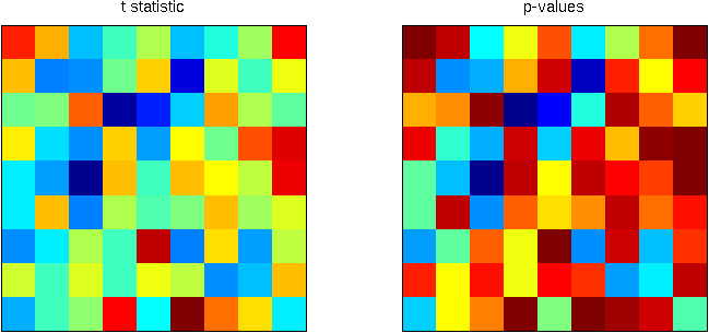
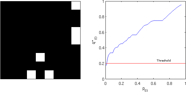
Consider the image below, on the left, a square of 9×9 pixels containing each some t-statistic with some sparse, low magnitude signal added. On the right are the corresponding p-values, ranging approximately between 0-1:

Statistical maps

Statistic and p-values

colorscale

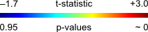
Using the B&H procedure to compute the threshold, with $q=0.20$ , and applying this threshold to the image rejects the null hypothesis in 6 pixels. On the right panel, the red line corresponds to the threshold. All p-values (in blue) below this line are declared significant.

FDR-threshold

FDR-threshold

Computing the FDR-corrected values at each pixel, and thresholding at the same $q=0.20$ , however, does not produce the same results, and just 1 pixel is declared significant. Although conservative, the “correction” is far from the nominal false discovery rate and is not appropriate. Note on the right panel the lack of monotonicity.

FDR-corrected

FDR-corrected

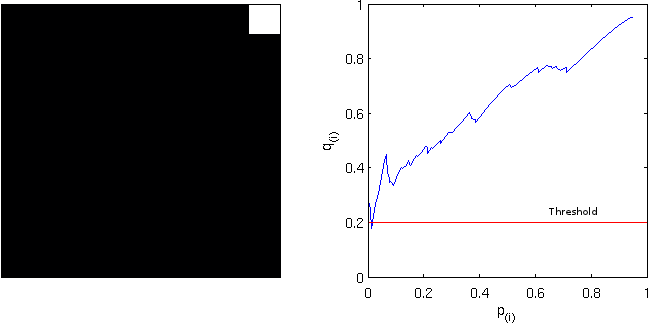
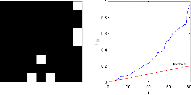
Computing instead the FDR-adjusted values, and thresholding again at $q=0.20$ produces the same results as with the simpler FDR-threshold. The adjustment is, thus, more “correct” than the “corrected”. Observe, on the right panel, the monotonicity enforced.

FDR-adjusted

FDR-adjusted

Implementation

An implementation of the three styles of FDR for Octave/MATLAB is available here: fdr.m
SPM users will find a similar feature in the function spm_P_FDR.m.

References

- Benjamini Y and Hochberg Y. Controlling the False Discovery Rate: A Practical and Powerful Approach to Multiple Testing. J R Statist Soc B. 1995; 57(1):289-300.
- Yekutieli D and Benjamini Y. Resampling-based false discovery rate controlling multiple test procedures for correlated test statistics. J Stat Plan Infer. 1999; 82(1-2):171-96.
- Benjamini Y and Yekutieli D. The control of the false discovery rate in multiple testing under dependency. Ann Statist. 2001; 29(4):1165-88.
- Genovese CR, Lazar NA, Nichols T. Thresholding of statistical maps in functional neuroimaging using the false discovery rate. Neuroimage. 2002 Apr;15(4):870-8.