
A Bernoulli trial is an experiment in which the outcome can be one of two mutually exclusive results, e.g. true/false, success/failure, heads/tails and so on. A number of methods are available to compute confidence intervals after many such trials have been performed. The most common have been discussed and reviewed by Brown et al. (2001), and are presented below. Consider 


Wald
This is the most common method, discussed in many textbooks, and probably the most problematic for small samples. It is based on a normal approximation to the binomial distribution, and it is often called “Wald interval” for it’s relationship with the Wald test. The interval is calculated as:
- Lower bound:
- Upper bound:


where 


Wald confidence interval.
Wilson
This interval appeared in Wilson (1927) and is defined as:
- Lower bound:
- Upper bound:


where 


Wilson confidence interval.
Agresti-Coull
This interval appeared in Agresti and Coull (1998) and shares many features with the Wilson interval. It is defined as:
- Lower bound:
- Upper bound:


where 

Agresti-Coull confidence interval.
Jeffreys
This interval has a Bayesian motivation and uses the Jeffreys prior (Jeffreys, 1946). It seems to have been introduced by Brown et al. (2001). It is defined as:
- Lower bound:
- Upper bound:


where 


Jeffreys confidence interval.
Clopper-Pearson
This interval was proposed by Clopper and Pearson (1934) and is based on a binomial test, rather than on approximations, hence sometimes being called “exact”, although it is not “exact” in the common sense. It is considered overly conservative.
- Lower bound:
- Upper bound:


where

Clopper-Pearson confidence interval.
Arc-Sine
This interval is based on the arc-sine variance-stabilising transformation. The interval is defined as:
- Lower bound:
- Upper bound:


where 


Arc-sine confidence interval.
Logit
This interval is based on the Wald interval for 
- Lower bound:
- Upper bound:


where 


Logit confidence interval.
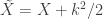
Anscombe
This interval was proposed by Anscombe (1956) and is based on the logit interval:
- Lower bound:
- Upper bound:
The difference is that 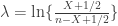
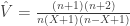


Anscombe’s confidence interval.
Octave/MATLAB implementation
A function that computes these intervals is available here: confint.m.
References
- Agresti A and Coull BA. Approximate is better than “exact” for interval estimation of binomial proportions. The American Statistician. 1998; 52(2):119-126.
- Anscombe FJ The transformation of Poisson, binomial and negative-binomial data. Biometrika. 1948; 35(3/4:246-254.
- Anscombe FJ. On estimating binomial response relations. Biometrika. 1956; 43(3/4):461-464.
- Brown LD, Cai TT, DasGupta A. Interval estimation for a binomial proportion. Statist Sci. 2001; 16(2):101-133.
- Clopper CJ, Pearson ES. The use of confidence or fiducial limits illustrated in the case of the binomial. Biometrika. 1934; 26(4):404-413.
- Jeffreys H. An invariant form for the prior probability in estimation problems. Proc. R. Soc. Lond. A. 1946; 186(1007):453-461.
- Wilson EB. Probable inference, the law of succession, and statistical inference. J Am Stat Assoc. 1927; 22(158):209-21.
