Merging multiple surfaces

Posted on 11.July.2013 by A. M. Winkler

Say you have a number of meshes in FreeSurfer ascii format (with extension *.asc or *.srf), one brain structure per file. However, for later processing or to import in some computer graphics software, you would like to have these multiple meshes all in a single file. This post provides a small script to accomplish this: mergesrf.

To use it, right click and save the file above, make it executable and, ideally, put it in a place where it can be found (or add its location to the environmental variable ${PATH}. Then run something as:

mergesrf file1.srf file2.srf fileN.srf mergedfile.srf

In this example, the output file is saved as mergedfile.srf. Another example is to convert all subcortical structures into just one large object, after aseg2srf as described here. To convert all, just change the current directory to ${SUBJECTS_DIR}//ascii, then run:

mergesrf * aseg_all.srf

A list with the input files and the output at the end is shown below:

The script uses Octave, which can be downloaded freely. The same script, with a small modification, can also run from inside matlab. This other version can be downloaded here: mergesrf.m

Requirements

In addition to Octave (or matlab), the script also requires functions to read and write surface files, which are available from the areal package (described here and downloadable here).

Biased, as it should be

Posted on 12.April.2013 by A. M. Winkler

When we run a permutation test, what we do is to first compute the statistic for the unpermuted model, then shuffle the data randomly, compute a new statistic and, if it is larger than the statistic for the unpermuted model, increment a counter. We then repeat the random shuffling, and keep incrementing the counter until we think we are done with them. We then divide the counter by the number of permutations and the result is the p-value what we wanted to find.

This procedure can be stated as:

$\hat{p} = \frac{1}{N}\sum^{N}_{n=1}\mathcal{I}(T^{*}_{n} \geqslant T_0)$

where $\hat{p}$ is the estimated p-value, $N$ is the number of permutations, $T_0$ is the statistic for the unpermuted model, $T^{*}_n$ is the statistic for the $n$ -th random shuffling, and $\mathcal{I}$ is an indicator function that evaluates as 1 if the condition between parenthesis is true, or 0 otherwise. This formulation produces unbiased results: since $E(\mathcal{I}(T^{*}_{n} \geqslant T_0)) = p$ , the true p-value, then $E(\frac{1}{N}\sum^{N}_{n=1}\mathcal{I}(T^{*}_{n} \geqslant T_0)) = p$ .

The problem

This strategy, however, has a problem. If the true p-value, $p$ , is small, or if the number of permutations is not sufficiently large, even after all the $N$ permutations are done, no $T^{*}_{n}$ may reach or surpass the value of $T_0$ , resulting in a p-value equal to 0. While this is still a valid, unbiased result, p-values equal to zero are problematic, as they can be interpreted as indicating the rejection of the null-hypothesis with absolute confidence. And this even after very few permutations (perhaps just 1!) have been performed, which is indeed rather counter-intuitive. We cannot be completely sure of the rejection of the null simply for having done just a few permutations.

Biasing to solve the problem

The solution is to make two modifications to the formulation above: start counting the $n$ -th permutation at 0, for the unpermuted model, and divide the counter at the end not by $N$ , but by $N+1$ :

$\hat{p} = \frac{1}{N+1}\sum^{N}_{n=0}\mathcal{I}(T^{*}_{n} \geqslant T_0)$

This formulation, which pools the unpermuted model together with the permuted realisations, is biased: for $n=0$ , $\mathcal{I}(T^{*}_{n} \geqslant T_0) = 1$ , and so, $E(\frac{1}{N+1}\sum^{N}_{n=0}\mathcal{I}(T^{*}_{n} \geqslant T_0)) = \frac{1+Np}{N+1} \neq p$ .

Quantifying the bias

The bias is smaller for a large number of permutations, and converges to zero as $N$ increases towards infinity. What is important, however, is that the bias punishes the results towards conservativeness whenever the true and unknown $p$ is smaller than $\frac{1}{N+1}$ , in a way that no p-value smaller than $\frac{1}{N+1}$ can ever be attained. It forces the researcher to run more permutations to find such small p-values to reject the null hypothesis, which otherwise could be rejected with a p-value equal to zero that would appear easily even after just a handful of permutations.

The bias is larger for smaller number of permutations and for smaller true p-values.

Controversy

The solution has been proposed by some authors, such as Edgington (1995), and strongly advocated by, e.g., Phipson and Smyth (2010). While the biased solution is definitely the most adequate for practical scientific problems, it can be considered as of little actual statistical meaning. Pesarin and Salmaso (2010) explain that the distribution of $T_0$ is not the same as the distribution of $T^{*}_{n}$ , unless the null is true. Under the alternative hypothesis, therefore, $T_0$ should not be pooled into the empirical distribution from which the p-value is obtained. Moreover, under the null, all possible permutations have the same probability, with no intrinsic reason to treat some (as the unpermuted) differently than others. If one wants unbiased results, the alternative formulation should obviously not be used.

References

Edgington ES. Randomization Tests. 3rd ed. Dekker, 1995.
Pesarin F and Salmaso L. Permutation Tests for Complex Data. Wiley, 2010.
Phipson B and Smith GK. Permutation P-values should never be zero: calculating exact P-values when permutations are randomly drawn. Stat Appl Genet Mol Biol. 2010;9:Article39.

Brain meshes available

Posted on 11.March.2013 by A. M. Winkler

A set of 3D brain meshes produced with FreeSurfer and individually partitioned into separate files following the atlases of Desikan-Killiany, Destrieux et al., and Desikan-Killiany-Tourville (DKT), is now available for download here. Surfaces for subcortical structures are also available.

These meshes are meant to be used to help with scientific visualisation and/or artistic rendering in computer graphics software, most prominently Blender, but also in any other application that can import files in Wavefront (*.obj) or Stanford Polygon (*.ply) formats. The released files are under a Creative Commons license. See the download page for details.

Competition ranking and empirical distributions

Posted on 28.November.2012 by A. M. Winkler

Estimating the empirical cumulative distribution function (empirical cdf) from a set of observed values requires computing, for each value, how many of the other values are smaller or equal to it. In other words, let $X = \{x_1, x_2, \ldots , x_N\}$ be the observed values, then:

$F(x) = P(X \leqslant x) = \frac{1}{N} \sum_{n=1}^{N}I(x_n \leqslant x)$

where $F(x)$ is the empirical cdf, $P(X \leqslant x)$ is the probability of observing a value in $X$ that is smaller than or equal to $x$ , $I(\cdot)$ is a function that evaluates as 1 if the condition in the parenthesis is satisfied or 0 otherwise, and $N$ is the number of observations. This definition is straightforward and can be found in many statistical textbooks (see, e.g., Papoulis, 1991).

For continuous distributions, a p-value for a given $x \in X$ can be computed as $1-F(x)$ . For a discrete cdf, however, this trivial relationship does not hold. The reason is that, while for continuous distributions the probability $P(X = x) = 0$ , for discrete distributions (such as empirical distributions), $P(X = x) > 0$ whenever $x \in X$ . As we often want to assign a probability to one of the values that have been observed, the condition $x \in X$ always holds, and the simple relationship between the cdf and the p-value is lost. The solution, however, is still simple: a p-value can be obtained from the cdf as $1-F(x) + 1/N$ .

In the absence of repeated values (ties), the cdf can be obtained computationally by sorting the observed data in ascending order, i.e., $X_{s} = \{x_{(1)}, x_{(2)}, \ldots , x_{(N)}\}$ . Then $F(x)=(n_x)/N$ , where $(n_x)$ represents the ascending rank of $x$ . Likewise, the p-value can be obtaining by sorting the data in descending order, and using a similar formula, $P(X \geqslant x) = (\tilde{n}_x)/N$ , where $(\tilde{n}_x)$ represents the descending rank of $x$ .

Example 1: Consider the following sequence of 10 observed values, already sorted in ascending order:

$X=\{75, 76, 79, 80, 84, 85, 86, 88, 90, 94\}$

The corresponding ranks are simply 1, 2, 3, 4, 5, 6, 7, 8, 9, 10. Consequently, the cdf is:

$F(x|x\in X) = \{0.1, 0.2, 0.3, 0.4, 0.5, 0.6, 0.7, 0.8, 0.9, 1\}$

The p-values are computed by using the ranks in descending order, i.e., 10, 9, 8, 7, 6, 5, 4, 3, 2, 1, which yields:

$P(X \geqslant x | x \in X) = \{1, 0.9, 0.8, 0.7, 0.6, 0.5, 0.4, 0.3, 0.2, 0.1\}$

The problem with ties

Simple sorting, as above, is effective when there are no repeated values in the data. However, in the presence of ties, simple sorting that produces ordinal rankings yield incorrect results.

Example 2: Consider the following sequence of 10 observed values, in which ties are present:

$X = \{81, 81, 82, 83, 83, 83, 84, 85, 85, 85\}$

If the same computational strategy discussed above were used, the we would conclude that the p-value for $x=85$ would be either 0.1, 0.2 or 0.3, depending on which instance of the “85” we were to choose. The correct value, however, is 0.3 (only), since 3 out of 10 variables are equal or above 85. The solution to this problem is to replace the simple, ordinal ranking, for a modified version of the so called competition ranking.

The competition ranking

The competition ranking assigns the same rank to values that are identical. The standard competition ranking for the previous sequence is, in ascending order, 1, 1, 3, 4, 4, 4, 7, 8, 8, 8. In descending order, the ranks are 9, 9, 8, 5, 5, 5, 4, 1, 1, 1. Note that in this ranking, the ties receive the “best” possible rank. A slightly different approach consists in assigning the “worst” possible rank to the ties. This modified competition ranking applied the previous sequence gives, in ascending order, the ranks 2, 2, 3, 5, 5, 5, 7, 10, 10, 10, whereas in descending order, the ranks are 10, 10, 8, 7, 7, 7, 4, 3, 3, 3.

Competition ranking solves the problem with ties for both the empirical cdf and for the calculation of the p-values. In both cases, it is the modified version of the ranking that needs to be used, i.e., the ranking that assigns the worst rank to identical values. Still using the same sequence as example, the cdf is given by:

$F(x|x\in X) = \{0.2, 0.2, 0.3, 0.6, 0.6, 0.6, 0.7, 1, 1, 1\}$

and the p-values are given by:

$P(X \geqslant x | x \in X) = \{1, 1, 0.8, 0.7, 0.7, 0.7, 0.4, 0.3, 0.3, 0.3\}$

Note that, as in the case with no ties, the p-values cannot be computed simply as $1-F(x)$ from the cdf as it would for continuous distributions. The correct formula is $1-F(x)+(n_x)/N$ , with $(n_x)$ here representing the frequency of $x$ .

Uses

The cdf of a set of observed data is useful in many types of non-parametric inference, particularly those that use bootstrap, jack-knife, Monte Carlo, or permutation tests. Ties can be quite common when working with discrete data and discrete explanatory variables using any of these methods.

Competition ranking in MATLAB and Octave

A function that computes the competition ranks for Octave and/or MATLAB is available to download here: csort.m.

Once installed, type help csort to obtain usage information.

References

Papoulis A. Probability, Random Variables and Stochastic Processes. McGraw-Hill, New York, 3rd ed, 1991.

The NIFTI file format

Posted on 23.September.2012 by A. M. Winkler

(This article is about the nifti-1 file format. For an overview of how the nifti-2 differs from the nifti-1, see this one.)

The Neuroimaging Informatics Technology Initiative (nifti) file format was envisioned about a decade ago as a replacement to the then widespread, yet problematic, analyze 7.5 file format. The main problem with the previous format was perhaps the lack of adequate information about orientation in space, such that the stored data could not be unambiguously interpreted. Although the file was used by many different imaging software, the lack of adequate information on orientation obliged some, most notably spm, to include, for every analyze file, an accompanying file describing the orientation, such as a file with extension .mat. The new format was defined in two meetings of the so called Data Format Working Group (dfwg) at the National Institutes of Health (nih), one in 31 March and another in 02 September of 2003. Representatives of some of the most popular neuroimaging software agreed upon a format that would include new information, and upon using the new format, either natively, or have it as an option to import and export.

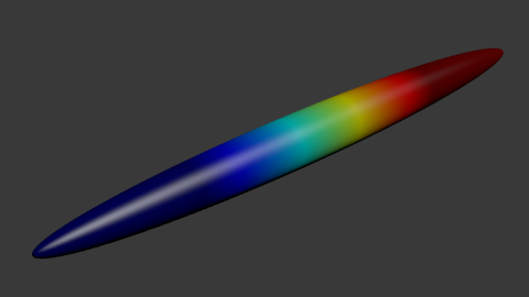
Radiological or “neurological”?

Perhaps the most visible consequence of the lack of orientation information was the then reigning confusion between left and right sides of brain images during the years in which the analyze format was dominant. It was by this time that researchers became used to describe an image as being in “neurological” or in “radiological” convention. These terms have always been inadequate because, in the absence of orientation information, no two pieces of software necessarily would have to display the same file with the same side of the brain in the same side of the screen. A file could be shown in “neurological” orientation in one software, but in radiological orientation in another, to the dismay of an unaware user. Moreover, although there is indeed a convention adopted by virtually all manufacturers of radiological equipment to show the left side of the patient on the right side of the observer, as if the patient were being observed from face-to-face or, if lying supine, from the feet, it is not known whether reputable neurologists ever actually convened to create a “neurological” convention that would be just the opposite of the radiological. The way as radiological exams are normally shown reflects the reality of the medical examination, in which the physician commonly approaches the patient in the bed from the direction of the feet (usually there is a wall behind the bed), and tend to stay face-to-face most of the time. Although the neurological examination does indeed include a few manoeuvres performed at the back, for most of the time, even in the more specialised semiotics, the physician stays at the front. The nifti format obviated all these issues, rendering these terms obsolete. Software can now mark the left or the right side correctly, sometimes giving the option of showing it flipped to better adapt to the user personal orientation preference.

Same format, different presentations

A single image stored in the analyze 7.5 format requires two files: a header, with extension .hdr, to store meta-information, and the actual data, with extension .img. In order to keep compatibility with the previous format, data stored in nifti format also uses a pair of files, .hdr/.img. Care was taken so that the internal structure of the nifti format would be mostly compatible with the structure of the analyze format. However, the new format added some clever improvements. Work with a pair of files for each image as in the .hdr/.img, rather than just one, is not only inconvenient, but it is also error prone, as one might easily forget (or not know) that the data of interest is actually split across more than one file. To address this issue, the nifti format also allows for storage as a single file, with extension .nii. Single file or pair of files are not the only possible presentations, though. It is very common for images to have large areas of solid background, or files describing masks and regions of interest containing just a few unique values that appear repeated many times. Files like these occupy large space in the disk, but with little actual information content. This is the perfect case where compression can achieve excellent results. Indeed, both nifti and analyze files can be compressed. The deflate algorithm (used, e.g., by gzip) can operate in streams, allowing compression and decompression on-the-fly. The compressed versions have the .gz extension appended: .nii.gz (single file) or .hdr/.img.gz (pair of files, either nifti or analyze).

Predefined dimensions for space and time

In the nifti format, the first three dimensions are reserved to define the three spatial dimensions — x, y and z —, while the fourth dimension is reserved to define the time points — t. The remaining dimensions, from fifth to seventh, are for other uses. The fifth dimension, however, can still have some predefined uses, such as to store voxel-specific distributional parameters or to hold vector-based data.

Overview of the header structure

In order to keep compatibility with the analyze format, the size of the nifti header was maintained at 348 bytes as in the old format. Some fields were reused, some were preserved, but ignored, and some were entirely overwritten. The table below shows each of the fields, their sizes, and a brief description. More details on how each field should be interpreted are provided further below.

Type	Name	Offset	Size	Description
`int`	`sizeof_hdr`	0B	4B	Size of the header. Must be 348 (bytes).
`char`	`data_type[10]`	4B	10B	Not used; compatibility with analyze.
`char`	`db_name[18]`	14B	18B	Not used; compatibility with analyze.
`int`	`extents`	32B	4B	Not used; compatibility with analyze.
`short`	`session_error`	36B	2B	Not used; compatibility with analyze.
`char`	`regular`	38B	1B	Not used; compatibility with analyze.
`char`	`dim_info`	39B	1B	Encoding directions (phase, frequency, slice).
`short`	`dim[8]`	40B	16B	Data array dimensions.
`float`	`intent_p1`	56B	4B	1st intent parameter.
`float`	`intent_p2`	60B	4B	2nd intent parameter.
`float`	`intent_p3`	64B	4B	3rd intent parameter.
`short`	`intent_code`	68B	2B	nifti intent.
`short`	`datatype`	70B	2B	Data type.
`short`	`bitpix`	72B	2B	Number of bits per voxel.
`short`	`slice_start`	74B	2B	First slice index.
`float`	`pixdim[8]`	76B	32B	Grid spacings (unit per dimension).
`float`	`vox_offset`	108B	4B	Offset into a .nii file.
`float`	`scl_slope`	112B	4B	Data scaling, slope.
`float`	`scl_inter`	116B	4B	Data scaling, offset.
`short`	`slice_end`	120B	2B	Last slice index.
`char`	`slice_code`	122B	1B	Slice timing order.
`char`	`xyzt_units`	123B	1B	Units of pixdim[1..4].
`float`	`cal_max`	124B	4B	Maximum display intensity.
`float`	`cal_min`	128B	4B	Minimum display intensity.
`float`	`slice_duration`	132B	4B	Time for one slice.
`float`	`toffset`	136B	4B	Time axis shift.
`int`	`glmax`	140B	4B	Not used; compatibility with analyze.
`int`	`glmin`	144B	4B	Not used; compatibility with analyze.
`char`	`descrip[80]`	148B	80B	Any text.
`char`	`aux_file[24]`	228B	24B	Auxiliary filename.
`short`	`qform_code`	252B	2B	Use the quaternion fields.
`short`	`sform_code`	254B	2B	Use of the affine fields.
`float`	`quatern_b`	256B	4B	Quaternion b parameter.
`float`	`quatern_c`	260B	4B	Quaternion c parameter.
`float`	`quatern_d`	264B	4B	Quaternion d parameter.
`float`	`qoffset_x`	268B	4B	Quaternion x shift.
`float`	`qoffset_y`	272B	4B	Quaternion y shift.
`float`	`qoffset_z`	276B	4B	Quaternion z shift.
`float`	`srow_x[4]`	280B	16B	1st row affine transform
`float`	`srow_y[4]`	296B	16B	2nd row affine transform.
`float`	`srow_z[4]`	312B	16B	3rd row affine transform.
`char`	`intent_name[16]`	328B	16B	Name or meaning of the data.
`char`	`magic[4]`	344B	4B	Magic string.
Total size			348B

Each of these fields is described in mode detail below, in the order as they appear in the header.

Size of the header

The field int sizeof_hdr stores the size of the header. It must be 348 for a nifti or analyze format.

Dim info

The field char dim_info stores, in just one byte, the frequency encoding direction (1, 2 or 3), the phase encoding direction (1, 2 or 3), and the direction in which the volume was sliced during the acquisition (1, 2 or 3). For spiral sequences, frequency and phase encoding are both set as 0. The reason to collapse all this information in just one byte was to save space. See also the fields short slice_start, short slice_end, char slice_code and float slice_duration.

Image dimensions

The field short dim[8] contains the size of the image array. The first element (dim[0]) contains the number of dimensions (1-7). If dim[0] is not in this interval, the data is assumed to have opposite endianness and so, should be byte-swapped (the nifti standard does not specify a specific field for endianness, but encourages the use of dim[0] for this purpose). The dimensions 1, 2 and 3 are assumed to refer to space (x, y, z), the 4th dimension is assumed to refer to time, and the remaining dimensions, 5, 6 and 7, can be anything else. The value dim[i] is a positive integer representing the length of the i-th dimension.

Intent

The short intent_code is an integer that codifies that the data is supposed to contain. Some of these codes require extra-parameters, such as the number of degrees of freedom (df). These extra parameters, when needed, can be stored in the fields intent_p* when they can be applied to the image as a while, or in the 5th dimension if voxelwise. A list of intent codes is in the table below:

Intent	Code	Parameters
None	`0`	no parameters
Correlation	`2`	p1 = degrees of freedom (df)
t test	`3`	p1 = df
F test	`4`	p1 = numerator df, p2 = denominator df
z score	`5`	no parameters
$\chi^2$ statistic	`6`	p1 = df
Beta distribution	`7`	p1 = a, p2 = b
Binomial distribution	`8`	p1 = number of trials, p2 = probability per trial
Gamma distribution	`9`	p1 = shape, p2 = scale
Poisson distribution	`10`	p1 = mean
Normal distribution	`11`	p1 = mean, p2 = standard deviation
Noncentral F statistic	`12`	p1 = numerator df, p2 = denominator df, p3 = numerator noncentrality parameter
Noncentral $\chi^2$ statistic	`13`	p1 = dof, p2 = noncentrality parameter
Logistic distribution	`14`	p1 = location, p2 = scale
Laplace distribution	`15`	p1 = location, p2 = scale
Uniform distribution	`16`	p1 = lower end, p2 = upper end
Noncentral t statistic	`17`	p1 = dof, p2 = noncentrality parameter
Weibull distribution	`18`	p1 = location, p2 = scale, p3 = power
$\chi$ distribution	`19`	p1 = df*
Inverse Gaussian	`20`	p1 = $\mu$ , p2 = $\lambda$
Extreme value type I	`21`	p1 = location, p2 = scale
p-value	`22`	no parameters
-ln(p)	`23`	no parameters
-log(p)	`24`	no parameters

* Note: For the $\chi$ distribution, when p1=1, it is a “half-normal” distribution; when p1=2, it is a Rayleigh distribution; and when p1=3, it is a Maxwell-Boltzmann distribution. Other intent codes are available to indicate that the file contains data that is not of statistical nature.

Intent	Code	Description
Estimate	`1001`	Estimate of some parameter, possibly indicated in `intent_name`
Label	`1002`	Indices of a set of labels, which may be indicated in `aux_file`.
NeuroName	`1003`	Indices in the NeuroNames set of labels.
Generic matrix	`1004`	For a MxN matrix in the 5th dimension, row major. p1 = M, p2 = N (integers as `float`); `dim[5]` = M*N.
Symmetric matrix	`1005`	For a symmetric NxN matrix in the 5th dimension, row major, lower matrix. p1 = N (integer as `float`); `dim[5]` = N*(N+1)/2.
Displacement vector	`1006`	Vector per voxel, stored in the 5th dimension.
Vector	`1007`	As above, vector per voxel, stored in the 5th dimension.
Point set	`1008`	Points in the space, in the 5th dimension. `dim[1]` = number of points; `dim[2]`=`dim[3]`=1; `intent_name` may be used to indicate modality.
Triangle	`1009`	Indices of points in space, in the 5th dimension. `dim[1]` = number of triangles.
Quaternion	`1010`	Quaternion in the 5th dimension.
Dimless	`1011`	Nothing. The intent may be in `intent_name`.
Time series	`2001`	Each voxel contains a time series.
Node index	`2002`	Each voxel is an index of a surface dataset.
rgb	`2003`	rgb triplet in the 5th dimension. `dim[0]` = 5, `dim[1]` has the number of entries, `dim[2:4]` = 1, `dim[5]` = 3.
rgba	`2004`	rgba quadruplet in the 5th dimension. `dim[0]` = 5, `dim[1]` has the number of entries, `dim[2:4]` = 1, `dim[5]` = 4.
Shape	`2005`	Value at each location is a shape parameter, such as a curvature.

The intent parameters are stored in the fields float intent_p1, float intent_p2 and float intent_p3. Alternatively, if the parameters are different for each voxel, they should be stored in the 5th dimension of the file. A human readable intent name can be stored in the field char intent_name[16], which may help to explain the intention of the data when it cannot or is not coded with any of the intent codes and parameters above.

Data type and bits per pixel/voxel

The field int datatype indicates the type of the data stored. Acceptable values are:

Type	Bitpix	Code
unknown	–	`0`
bool	1 bit	`1`
unsigned char	8 bits	`2`
signed short	16 bits	`4`
signed int	32 bits	`8`
float	32 bits	`16`
complex	64 bits	`32`
double	64 bits	`64`
rgb	24 bits	`128`
“all”	–	`255`
signed char	8 bits	`256`
unsigned short	16 bits	`512`
unsigned int	32 bits	`768`
long long	64 bits	`1024`
unsigned long long	64 bits	`1280`
long double	128 bits	`1536`
double pair	128 bits	`1792`
long double pair	256 bits	`2048`
rgba	32 bits	`2304`

The field short bitpix holds the information of the number of bits per voxel. The value must match the type determined by datatype as shown above.

Slice acquisition information

The fields fields char slice_code, short slice_start, short slice_end and float slice_duration are useful to store information about the timing of an fMRI acquisition, and need to be used together with the char dim_info, which contains the field slice_dim. If, and only if, the slice_dim is different than zero, slice_code is interpreted as:

Code	Interpretation
`0`	Slice order unknown
`1`	Sequential, increasing
`2`	Sequential, decreasing
`3`	Interleaved, increasing, starting at the 1st mri slice
`4`	Interleaved, decreasing, starting at the last mri slice
`5`	Interleaved, increasing, starting at the 2nd mri slice
`6`	Interleaved, decreasing, starting at one before the last mri slice

The fields short slice_start and short slice_end inform respectively which are the first the last slices that correspond to the actual mri acquisition. Slices present in the image that are outside this range are treated as padded slices (for instance, containing zeroes). The field float slice_duration indicates the amount of time needed to acquire a single slice. Having this information in a separate field allows to correctly store images of experiments in which slice_duration*dim[slice_dim] is smaller than the value stored in pixdim[4], usually the repetition time (tr).

Slice codes to specify slice acquisition timings. In this example, slice_start = 2 and slice_end = 11, indicating that slices #01 and #12 stored in the file have not been truly acquired with MRI, but instead, were padded to the file. The field slice_duration specifies how long it took to acquire each slice. The dimension that corresponds to the slice acquisition (in this case dim[3], z) is encoded in the field dim_info.

Voxel dimensions

The dimension for each voxel is stored in the field float pixdim[8], and each element match its respective in short dim[8]. The value in float pixdim[0], however, has a special meaning, discussed below; it should always be -1 or 1. The units of measurement for the first 4 dimensions are specified in the field xyzt_units, discussed below.

Voxel offset

The field int vox_offset indicates, for single files (.nii), the byte offset before the imaging data starts. For compatibility with older software, possible values are multiples of 16, and the minimum value is 352 (the smallest multiple of 16 that is larger than 348). For file pairs (.hdr/.img), this should be set as zero if no information other than image data itself is to be stored in the .img (most common), but it can also be larger than zero, allowing for user-defined extra-information to be prepended into the .img, such as a dicom header. In this case, however, the rule of being a multiple of 16 may eventually be violated. This field is of type float (32-bit, ieee-754), allowing integers up to 2²⁴ to be specified. The reason for using float rather than what would be the more natural choice, int, is to allow compatibility with the analyze format.

Data scaling

The values stored in each voxel can be linearly scaled to different units. The fields float scl_slope and float scl_inter define a slope and an intercept for a linear function. The data scaling feature allows the storage in a wider range than what would be allowed by the datatype. Yet, it is possible to use scaling within the same datatype. Both scaling fields should be ignored for the storage of rgb data. For complex types, it should be applied to both real and imaginary parts.

Data display

For files that store scalar (non-vector) data, the fields float cal_min and float cal_max determine the intended display range when the image is opened. Voxel values equal or below cal_min should be shown with the smallest colour in the colourscale (typically black in a gray-scale visualisation), and values equal or above cal_max should be shown with the largest colour in the colourscale (typically white).

Measurement units

Both spatial and temporal measurement units, used for the dimensions dim[1] to dim[4] (and, respectively, for pixdim[]), are encoded in the field char xyzt_units. The bits 1-3 are used to store the spatial dimensions, the bits 4-6 are for temporal dimensions, and the bits 6 and 7 are not used. A temporal offset can be specified in the field float toffset. The codes for xyzt_units, in decimal, are:

Unit	Code
Unknown	`0`
Meter (m)	`1`
Milimeter (mm)	`2`
Micron (µm)	`3`
Seconds (s)	`8`
Miliseconds (ms)	`16`
Microseconds (µs)	`24`
Hertz (Hz)	`32`
Parts-per-million (ppm)	`40`
Radians per second (rad/s)	`48`

Description

This field, char descrip[80] can contain any text with up to 80 characters. The standard does not specify whether this string needs to be terminated by a null character or not. Presumably, it is up to the application to correctly handle it.

Auxiliary file

A supplementary file, containing extra-information, can be specified in the field char aux_file[24]. This file can, for instance, contain the face indices for meshes which points are stored in the 5th dimension or a look-up-table to display colours.

Orientation information

The most visible improvement of the nifti format over the previous analyze format is the ability to unambiguously store information orientation. The file standard assumes that the voxel coordinates refer to the center of each voxel, rather than at any of its corners. The world coordinate system is assumed to be ras: +x is Right, +y is Anterior and +z is Superior, which is precisely different than the coordinate system used in analyze, which is las. The format provides three different methods to map the voxel coordinates (i,j,k) to the world coordinates (x,y,z). The first method exists only to allow compatibility with the analyze format. The other two methods may coexist, and convey different coordinate systems. These systems are specified in the fields short qform_code and short sform_code, which can assume the values specified in the table:

Name	Code	Description
unknown	`0`	Arbitrary coordinates. Use Method 1.
scanner_anat	`1`	Scanner-based anatomical coordinates.
aligned_anat	`2`	Coordinates aligned to another file, or to the “truth” (with an arbitrary coordinate center).
talairach	`3`	Coordinates aligned to the Talairach space.
mni_152	`4`	Coordinates aligned to the mni space.

In principle, the qform_code (Method 2 below) should contain either 0, 1 or 2, whereas the sform_code (Method 3 below) could contain any of the codes shown in the table.

Method 1

The Method 1 is for compatibility with analyze and is not supposed to be used as the main orientation method. The world coordinates are determined simply by scaling by the voxel size:

$\left[ \begin{array}{c} x\\ y\\ z \end{array} \right]= \left[ \begin{array}{c} i\\ j\\ k \end{array} \right]\odot \left[ \begin{array}{c} \mathtt{pixdim[1]}\\ \mathtt{pixdim[2]}\\ \mathtt{pixdim[3]}\\ \end{array} \right]$

where $\odot$ is the Hadamard product.

Method 2

The Method 2 is used when short qform_code is larger than zero, and is intended to be used to indicate the scanner coordinates, in a way that resembles the coordinates specified in the dicom header. It can also be used to represent the alignment of an image to a previous session of the same subject (such as for coregistration). For compactness and simplicity, the information in this field is stored as quaternions (a,b,c,d), which last three coefficients are in the fields float quatern_b, float quatern_c, float quatern_d. The first coefficient can be calculated from the other three as 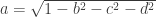$a = \sqrt{1-b^2-c^2-d^2}$ . These fields are used to construct a rotation matrix as:

$\mathbf{R} = \left[ \begin{array}{ccc} a^2+b^2-c^2-d^2 & 2(bc-ad) & 2(bd+ac) \\ 2(bc+ad) & a^2+c^2-b^2-d^2 & 2(cd-ab) \\ 2(bd-ac) & 2(cd+ab) & a^2+d^2-b^2-c^2 \end{array} \right]$

This rotation matrix, together with the voxel sizes and a translation vector, is used to define the final transformation from voxel to world space:

$\left[ \begin{array}{c} x\\ y\\ z \end{array} \right]=\mathbf{R} \left[ \begin{array}{c} i\\ j\\ q\cdot k\\ \end{array} \right]\odot \left[ \begin{array}{c} \mathtt{pixdim[1]}\\ \mathtt{pixdim[2]}\\ \mathtt{pixdim[3]}\\ \end{array} \right]+ \left[ \begin{array}{c} \mathtt{qoffset\_x}\\ \mathtt{qoffset\_y}\\ \mathtt{qoffset\_z}\\ \end{array} \right]$

where $\odot$ is, again, the Hadamard product, and $q$ is the qfac value, stored at the otherwise unused pixdim[0], which should be either -1 or 1. Any different value should be treated as 1.

Method 3

The Method 3 is used when short sform_code is larger than zero. It relies on a full affine matrix, stored in the header in the fields float srow_*[4], to map voxel to world coordinates:

$\left[ \begin{array}{c} x\\ y\\ z\\ 1 \end{array} \right]=\left[ \begin{array}{cccc} \mathtt{srow\_x[0]} & \mathtt{srow\_x[1]} & \mathtt{srow\_x[2]} & \mathtt{srow\_x[3]}\\ \mathtt{srow\_y[0]} & \mathtt{srow\_y[1]} & \mathtt{srow\_y[2]} & \mathtt{srow\_y[3]}\\ \mathtt{srow\_z[0]} & \mathtt{srow\_z[1]} & \mathtt{srow\_z[2]} & \mathtt{srow\_z[3]} \\ 0 & 0 & 0 & 1\end{array} \right]\cdot\left[ \begin{array}{c} i\\ j\\ k\\ 1 \end{array} \right]$

Differently than Method 2, which is supposed to contain a transformation that maps voxel indices to the scanner world coordinates, or to align between two distinct images of the same subject, the Method 3 is used to indicate the transformation to some standard world space, such as the Talairach or mni coordinates, in which case, the coordinate system has its origin (0,0,0) at the anterior comissure of the brain.

Magic string

The char magic[4] field is a “magic” string that declares the file as conforming with the nifti standard. It was placed at the very end of the header to avoid overwriting fields that are needed for the analyze format. Ideally, however, this string should be checked first. It should be 'ni1' (or '6E 69 31 00' in hexadecimal) for .hdr/.img pair, or 'n+1' (or '6E 2B 31 00') for a .nii single file. In the absence of this string, the file should be treated as analyze. Future versions of the nifti format may increment the string to 'n+2', 'n+3', etc. Indeed, as of 2012, a second version is under preparation.

Unused fields

The fields char data_type[10], char db_name[18], int extents, short session_error and char regular are not used by the nifti format, but were included in the header for compatibility with analyze. The extents should be the integer 16384, and regular should be the character 'r'. The fields int glmin and int glmax specify respectively the minimum and maximum of the entire dataset in the analyze format.

Storing extra-information

Extra information can be included in the nifti format in a number of ways as allowed by the standard. At the end of the header, the next 4 bytes (i.e., from byte 349 to 352, inclusive) may or may not be present in a .hdr file. However, these bytes will always be present in a .nii file. They should be interpreted as a character array, i.e. char extension[4]. In principle, these 4 bytes should be all set to zero. If the first, extension[0], is non-zero, this indicates the presence of extended information beginning at the byte number 353. Such extended information needs to have size multiple of 16. The first 8 bytes of this extension should be interpreted as two integers, int esize and int ecode. The field esize indicates the size of the extent, including the first 8 bytes that are the esize and ecode themselves. The field ecode indicates the format used for the remaining of the extension. At the time of this writing, three codes have been defined:

Code	Use
`0`	Unknown. This code should be avoided.
`2`	dicom extensions
`4`	xml extensions used by the afni software package.

More than one extension can be present in the same file, each one always starting with the pair esize and ecode, and with its first byte immediately past the last byte of the previous extension. In a single .nii file, the float vox_offset must be set properly so that the imaging data begins only after the end of the last extension.

Problems

The nifti format brought a number of great benefits if compared to the old analyze format. However, it also brought its own set of new problems. Fortunately, these problems are not severe. Here are some:

Even though a huge effort was done to keep compatibility with analyze, a crucial aspect was not preserved: the world coordinate system is assumed, in the nifti format, to be ras, which is weird and confusing. The las is a much more logical choice from a medical perspective. Fortunately, since orientation is stored unambiguously, it is possible to later flip the images in the screen at will in most software.
The file format still relies too much on the file extension being .nii or on a pair .hdr/.img, rather than much less ambiguous magic strings or numbers. On the other hand, the different magic strings for single file and for file pairs effectively prevent the possibility of file splitting/merging using common operating system tools (such as dd in Linux), as the magic string needs to be changed, even though the header structure remains absolutely identical.
The magic string that is present in the header is not placed at the beginning, but near its end, which makes the file virtually unrecognisable outside of the neuroimaging field.
The specification of three different coordinate systems, while bringing flexibility, also brought ambiguity, as nowhere in the standard there is information on which should be preferred when more than one is present. Certain software packages explicitly force the qform_code and sform_code to be identical to each other.
There is no field specifying a preferred interpolation method when using Methods 2 or 3, even though these methods do allow fractional voxels to be found with the specification of world coordinates.
Method 2 allows only rotation and translation, but sometimes, due to all sorts of scanner calibration issues and different kinds of geometric distortion present in different sequences, the coregistration between two images of the same subject may require scaling and shear, which are only provided in Method 3.
Method 3 is supposed to inform that the data is aligned to a standard space using an affine transformation. This works perfectly if the data has been previously warped to such a space. Otherwise, the simple alignment of any actual brain from native to standard space cannot be obtained with only linear transformations.
To squeeze information while keeping compatibility with the analyze format, some fields had to be mangled into just one byte, such as char dim_info and char xyzt_units, which is not practical and require sub-byte manipulation.
The field float vox_offset, directly inherited from the analyze format, should in fact, be an integer. Having it as a float only adds confusion.
Not all software packages implement the format exactly in the same way. Vector-based data, for instance, which should be stored in the 5th dimension, is often stored in the 4th, which should be reserved for time. Although this is not a problem with the format itself, but with the use made of it, easy implementation malpractices lead to a dissemination of ambiguous and ill-formed files that eventually cannot be read in other applications as intended by the time of the file creation.

Despite these issues, the format has been very successful as a means to exchange data between different software packages. An updated format, the nifti 2.0, with a header with more than 500 bytes of information, may become official soon. (UPDATE: details here)

More information

The official definition of the nifti format is available as a c header file (nifti1.h) here and mirrored here.

Brainder.org goes ad-free

Posted on 21.September.2012 by A. M. Winkler

Those annoying ads that were placed in some pages by the hosting service should be gone from now on. Brainder.org is now ad-free!

FLAIR templates available

Posted on 25.August.2012 by A. M. Winkler

A set of brain templates constructed using fluid-attenuated inverse recovery (FLAIR) images are now available for download here. These templates can be used, for instance, to help to automatically identify white matter hyperintensities (WMH; e.g. leukoaraiosis, multiple sclerosis) from magnetic resonance images (MRI), or as target for registration of other individual FLAIR images without the need of a matching T1-weighted image. Two versions are available, based on the full or on a restricted sample, each of these in three different resolutions (0.7 mm, 1.0 mm and 2.0 mm). In addition to FLAIR, templates for gray matter (GM), white matter (WM), cerebrospinal fluid (CSF) and T1-weighted (T1) are also provided. Follow the link above for more information and to download.

Automatic atlas queries in FSL

Posted on 30.July.2012 by A. M. Winkler

The fmrib Software Library (fsl) provides a tool to query whether regions belong or not to one of various atlases available. This well-known tool is called atlasquery, and it requires one region per image per run. To run for multiple separate regions on a single image image (e.g., a thresholded statistical map), a separate call to fsl‘s cluster command (not to be confused with the homonym cluster command that is part of the GraphViz package) is needed.

In order to automate this task, a small script called autoaq is available (UPDATE: the script is no longer supplied here; it has been incorporated into fsl). Usage information is provided by calling the command without arguments. This is the same script we posted recently to the fsl mailing list (here). Obviously, it does not run in Microsoft Windows. To use it, you need any recent Linux or Mac computer with fsl installed.

An example call is shown below:

./autoaq -i pvals.nii.gz -t 0.95 -o report.txt -a "JHU White-Matter Tractography Atlas"

The command will write temporary files to the directory from where it is called, hence it needs to be called from a directory to which the user has writing permissions. The atlas name can be any of the atlases available in fsl, currently being the ones listed below (note the quotes, ” “, that need to be provided when calling autoaq):

“Cerebellar Atlas in MNI152 space after normalization with FLIRT”
“Cerebellar Atlas in MNI152 space after normalization with FNIRT”
“Harvard-Oxford Cortical Structural Atlas”
“Harvard-Oxford Subcortical Structural Atlas”
“JHU ICBM-DTI-81 White-Matter Labels”
“JHU White-Matter Tractography Atlas”
“Juelich Histological Atlas”
“MNI Structural Atlas”
“Oxford Thalamic Connectivity Probability Atlas”
“Oxford-Imanova Striatal Connectivity Atlas 3 sub-regions”
“Oxford-Imanova Striatal Connectivity Atlas 7 sub-regions”
“Oxford-Imanova Striatal Structural Atlas”
“Talairach Daemon Labels”

The list can always be obtained through atlasquery --dumpatlases. Information about these atlases is available here.

The output is divided in three sections. In the first, a table containing the cluster indices, size and coordinates of the peaks and centres of mass is provided. In the second part, the structures to which the cluster peaks belong are presented, along with the associated probabilities. In the third part, probabilities for each cluster as a whole is presented. If the atlas is a binary label atlas, the number shown is in fact the overlap percentage between the cluster and the respective atlas label. If the atlas is probabilistic, the value is the mean probability in the overlapping region.

Version history:

03.Oct.2012: Update – Fixed issue with the md5 command under a different name in vanilla Mac.
25.Jan.2014: Update – Added options -u (to update/append a previous report) and -p to show peak coordinates instead of center of mass.
10.Dec.2014: The autoaq has been integrated into the freely available fmrib Software Library (fsl) and is no longer provided here. Hope you enjoy using it directly into fsl! :-)

Facewise brain cortical surface area: scripts now available

Posted on 02.June.2012 by A. M. Winkler

In the paper Measuring and comparing brain cortical surface area and other areal quantities (Neuroimage, 2012;61(4):1428-43, doi:10.1016/j.neuroimage.2012.03.026, pmid:22446492), we described the steps to perform pycnophylactic interpolation, i.e., mass-conservative interpolation, of brain surface area. The method is also valid for any other quantity that is also areal by nature.

The scripts to perform the steps we propose in the paper are now freely available for Octave and/or matlab. They can also be executed directly from the shell using Octave as the interpreter. In this case, multiple instances can be easily submitted to run in a cluster. Click here to dowload and for step-by-step instructions.

Retrospective motion correction for structural MRI

Posted on 17.May.2012 by A. M. Winkler

Good quality results can only be obtained with good quality images. To obtain images with good SNR and high resolution, long scan times are often necessary. However, with longer acquisition, the subjects are more likely to move. Rather than acquire a very long sequence, that often can last up to 40 minutes, the acquisition can be broken into many shorter scans, each with lower SNR. These are coregistered, effectively reducing the effect of undesired movement, and averaged, for increase of the SNR (Kochunov et al, 2006).

The last image in the second row is the average of all the other seven, after retrospective motion correction has been applied.

The results above are typical. Each pixel above corresponds to a true voxel, with no interpolation. Therefore, to see in more detail, simply download the image above and use an image viewer (e.g. gwenview or eog) to zoom.

The method is termed retrospective to discern it from prospective motion correction methods, such as those available for BOLD-sensitive EPI acquisitions (e.g. Siemens 3D PACE).

Since the images belong to the same subject and typically the movement is of only a few degrees or milimeters, the affine matrices for these corrections should have a diagonal with values very close to 1 and very close to zero off the diagonal. Here is one example:

0.999995    -0.00020007  -0.0030414    0.106906
0.000188555  0.999993    -0.00378601   0.100499
0.00304214   0.00378542   0.999988    -0.204133
0            0            0            1

As usual, the improvement in the SNR is given by a factor of $\sqrt{n}$ , where $n$ is the number of images averaged.

Download

A script to apply the method is available here: stereomc. Just download and make it executable. Call it without arguments to obtain usage information.