The logic of the Fisher method to combine P-values

Consider a set of k independent tests, each of these to test a certain null hypothesis \mathcal{H}_{0|i}, i=\{1, 2, \ldots, k\}. For each test, a significance level P_{i}, i.e., a p-value, is obtained. All these p-values can be combined into a joint test whether there is a global effect, i.e., if a global null hypothesis \mathcal{H}_0 can be rejected.

There are a number of ways to combine these independent, partial tests. The Fisher method is one of these, and is perhaps the most famous and most widely used. The test was presented in Fisher’s now classical book, Statistical Methods for Research Workers, and was described rather succinctly:

When a number of quite independent tests of significance have been made, it sometimes happens that although few or none can be claimed individually as significant, yet the aggregate gives an impression that the probabilities are on the whole lower than would often have been obtained by chance. It is sometimes desired, taking account only of these probabilities, and not of the detailed composition of the data from which they are derived, which may be of very different kinds, to obtain a single test of the significance of the aggregate, based on the product of the probabilities individually observed.
The circumstance that the sum of a number of values of \chi^{2} is itself distributed in the \chi^{2} distribution with the appropriate number of degrees of freedom, may be made the basis of such a test. For in the particular case when n=2, the natural logarithm of the probability is equal to \frac{1}{2}\chi^{2}. If therefore we take the natural logarithm of a probability, change its sign and double it, we have the equivalent value of \chi^{2} for 2 degrees of freedom. Any number of such values may be added together, to give a composite test, using the Table of \chi^{2} to examine the significance of the result. — Fisher, 1932.

The test is based on the fact that the probability of rejecting the global null hypothesis is related to intersection of the probabilities of each individual test, \prod_{i} P_{i}. However, \prod_{i} P_{i} is not uniformly distributed, even if the null is true for all partial tests, and cannot be used itself as the joint significance level for the global test. To remediate this fact, some interesting properties and relationships among distributions of random variables were exploited by Fisher and embodied in the succinct excerpt above. These properties are discussed below.

The logarithm of uniform is exponential

The cumulative distribution function (cdf) of an exponential distribution is:

F(x)=1- e^{-\lambda x}

where \lambda is the rate parameter, the only parameter of this distribution. The inverse cdf is, therefore, given by:

x = -\dfrac{1}{\lambda}\ln(1-F(x))

If P is a random variable uniformly distributed in the interval [0, 1], so is 1-P, and it is immaterial to differ between them. As a consequence, the previous equation can be equivalently written as:

x = -\dfrac{1}{\lambda}\ln(P)

where P \sim \mathcal{U}(0,1), which highlights the fact that the negative of the natural logarithm of a random variable distributed uniformly between 0 and 1 follows an exponential distribution with rate parameter \lambda=1.

An exponential with rate 1/2 is chi-squared

The cdf of a chi-squared distribution with \nu degrees of freedom, i.e. \chi^{2}_{\nu}, is given by:

F(x; \nu) = \dfrac{\int_{0}^{x/2} t^{\frac{\nu}{2}-1}e^{-t}{\rm d}t}{\left(\frac{\nu}{2}-1\right)!}

If \nu=2, and solving the integral we have:

F(x; \nu=2) = \dfrac{\int_{0}^{x/2} t^{\frac{2}{2}-1}e^{-t}{\rm d}t}{\left(\frac{2}{2}-1\right)!} = \int_{0}^{x/2} e^{-t}{\rm d}t = 1-e^{-x/2}

In other words, a \chi^{2} distribution with \nu=2 is equivalent to an exponential distribution with rate parameter \lambda=1/2.

The sum of chi-squared is also chi-squared

The moment-generating function (mgf) of a sum of independent variables is the product of the mgfs of the respective variables. The mgf of a \chi^{2}_{\nu} is:

M(t) = (1-2t)^{-\nu/2}

The mgf of the sum of k independent variables that follow each a \chi^{2}_{2} distribution is then given by:

M_{\text{sum}}(t) = \prod_{i=1}^{k} (1-2t)^{-2/2} = (1-2t)^{-k}

which also defines a \chi^{2} distribution, however with degrees of freedom \nu=2k.

Assembling the pieces

With these facts in mind, how to transform the product \prod_{i} P_{i} into a p-value that is uniformly distributed when the global null is true? The product can be converted into a sum by taking the logarithm. And as shown above, the logarithm of uniformly distributed variables follows an exponential distribution with rate parameter \lambda=1. Multiplication of each \ln(P_{i}) by 2 changes the rate parameter to \lambda=1/2 and makes this distribution equivalent to a \chi^{2} distribution with degrees of freedom \nu=2. The sum of k of these logarithms also follow a \chi^2 distribution, now with \nu=2k degrees of freedom, i.e., \chi^{2}_{2k}.

The statistic for the Fisher method is, therefore, computed as:

X = -2 \sum_{i=1}^{k} \ln(P_{i})

with X following a \chi^{2}_{2k} distribution, from which a p-value for the global hypothesis can be easily obtained.

Reference

The details above are not in the book, presumably omitted by Fisher as the knowledge of these derivation details would be of little practical use. Nonetheless, the reference for the book is:

See also

The Fisher’s method to combine p-values is one of the most powerful combining functions that can be used for Non-Parametric Combination.

Importing FreeSurfer subcortical structures into Blender

In a previous article, a method to import cortical meshes from FreeSurfer into Blender and other CG applications was presented. Here it is complemented with a method to import the subcortical structures. These structures are segmented as part of FreeSurfer subcortical stream, and are stored in a volume-based representation. In order to import into Blender, first it is necessary to generate surfaces, then convert to Wavefront OBJ, and finally, do the import. Below is an example of how the output looks like.

An example of a subcortical meshes generated from FreeSurfer subcortical segmentations imported into Blender.

Generating the surfaces for subcortical structures

The surfaces can be generated using FreeSurfer’s own tools. The script aseg2srf automates the task. Suppose you would like to create meshes for all subcortical structures of the subjects named “capitu”, “bentinho” and “ezequiel”. Simply run:

aseg2srf -s "capitu bentinho ezequiel"

The outputs are saved in a directory called ascii, inside each subject’s directory. The script requires that FreeSurfer is installed and working properly, and that the environmental variable ${SUBJECTS_DIR} has been set to point to the location where the subjects are. It is also necessary to have writing permissions to this directory, so that the surfaces can be saved.

If there are many subjects, provide a list from a text file, with one subject per line:

aseg2srf -s list.txt

To make surfaces for just some structures, provide their label numbers with the -l option. For the hippocampus, for instance, the labels are 17 and 53 for left and right respectively:

aseg2srf -s "capitu bentinho ezequiel" -l "17 53"

The script has also a -d option, for debugging, which allows to keep temporary files used during the mesh generation.

List of labels

Below is a list of the label codes for the major structures. A more comprehensive list is in the aseg.stats file, inside the stats directory for each subject, or in the FreeSurferColorLUT.txt file (in the FreeSurfer directory).

Left lateral ventricle 4
Left inferior part of the lateral ventricle 5
Left cerebellum white matter 7
Left cerebellum cortex 8
Left thalamus 10
Left caudate 11
Left putamen 12
Left pallidum 13
Left hippocampus 17
Left amygdala 18
CSF 24
Left accumbens 26
Left ventral diencephalon 28
Left choroid plexus 31
Right lateral ventricle 43
Right inferior part of the lateral ventricle 44
Right cerebellum white matter 46
Right cerebellum cortex 47
Right thalamus 49
Right caudate 50
Right putamen 51
Right pallidum 52
Right hippocampus 53
Right amygdala 54
Right accumbens 58
Right ventral diencephalon 60
Right choroid plexus 63
Corpus callosum, posterior part 251
Corpus callosum, middle posterior part 252
Corpus callosum, central part 253
Corpus callosum, middle anterior part 254
Corpus callosum, anterior part 255
3rd ventricle 14
4th ventricle 15
5th ventricle (CSF sometimes found in the septum pellucidum) 72
Brain stem 16

Conversion to Wavefront OBJ

Once the meshes have been generated, the process of conversion into a format that can be read by CG software is the same as described previously here.

Download

The script is available here: aseg2srf.

Requirements

FreeSurfer must be installed and working properly. The environmental variable ${SUBJECTS_DIR} must point to the directory where the data for each subject is located. It is also assumed that recon-all has been run successfully.

Importing FreeSurfer cortical meshes into Blender

Computer graphics (CG) applications, such as Blender, Maya or 3D Studio, doesn’t come with filters that allow to directly import or export FreeSurfer meshes. To import brain surfaces to these applications, converting first to an intermediate file format solves the problem. Below is an example of a brain imported into Blender.

An example of a brain mesh from FreeSurfer imported into Blender after conversion to Wavefront OBJ.

The mris_convert, from FreeSurfer, allows conversion to stereolithography format (STL). However, not all CG applications read natively from STL files. Moreover, other formats, such as Wavefront OBJ and Stanford PLY have simpler structure — yet allowing features that will be discussed here in forthcoming articles.

Conversion from FreeSurfer to Wavefront OBJ

A simple procedure to convert a FreeSurfer surface to Wavefront OBJ (ASCII) is:

1) Use mris_convert to convert from FreeSurfer binary to ASCII:

mris_convert lh.pial lh.pial.asc

2) A suggestion is to rename the .asc file to .srf, to differentiate it from other files that also have .asc extension and have a different internal structure.

mv lh.pial.asc lh.pial.srf

3) Use the script srf2obj to convert from .srf to .asc:

srf2obj lh.pial.srf > lh.pial.obj

The symbol “>” is necessary so that the output from srf2obj is redirected to a new file.

Conversion from Wavefront OBJ to FreeSurfer

To convert back to FreeSurfer, a similar strategy is used.

1) Use the script obj2srf to generate new .srf files (here directly named as .asc, as expected by mris_convert)

obj2srf lh.pial.obj > lh.pial.asc

2) Use mris_convert:

mris_convert lh.pial.asc lh.pial

Download

Both scripts are available here: srf2obj and obj2srf. Right-click and save, then make them executable.

Requirements

The scripts use gawk as the interpreter, and expects to find it on its usual location (/bin/gawk). If in your system gawk is installed elsewhere, modify the first line accordingly.

If you don’t have gawk, you can get it from the repository of your Linux distribution. For Mac, gawk is available in MacPorts and Fink. Alternatively, you may replace gawk with awk itself, nawk, or any other awk implementation that works.

Confidence intervals for Bernoulli trials

A Bernoulli trial is an experiment in which the outcome can be one of two mutually exclusive results, e.g. true/false, success/failure, heads/tails and so on. A number of methods are available to compute confidence intervals after many such trials have been performed. The most common have been discussed and reviewed by Brown et al. (2001), and are presented below. Consider n trials, with X successes and a significance level of \alpha=0.05 to obtain a 95% confidence interval. For each of the methods, the interval is shown graphically for 1 \leqslant n \leqslant 100 and 1 \leqslant X \leqslant n.

Wald

This is the most common method, discussed in many textbooks, and probably the most problematic for small samples. It is based on a normal approximation to the binomial distribution, and it is often called “Wald interval” for it’s relationship with the Wald test. The interval is calculated as:

  • Lower bound: L=p-k\sqrt{pq/n}
  • Upper bound: U=p+k\sqrt{pq/n}

where k = \Phi^{-1}\{1-\alpha/2\}, \Phi^{-1} is the probit function, p=X/n and q=1-p.

Wald confidence interval.

Wilson

This interval appeared in Wilson (1927) and is defined as:

  • Lower bound: L = \tilde{p} - (k/\tilde{n})\sqrt{npq+k^2/4}
  • Upper bound: U = \tilde{p} + (k/\tilde{n})\sqrt{npq+k^2/4}

where \tilde{p} = \tilde{X}/\tilde{n}, \tilde{n}=n+k^2, \tilde{X} = X+ k^2/2, and the remaining are as above. This is probably the most appropriate for the majority of situations.

Wilson confidence interval.

Agresti-Coull

This interval appeared in Agresti and Coull (1998) and shares many features with the Wilson interval. It is defined as:

  • Lower bound: L = \tilde{p} - k\sqrt{\tilde{p}\tilde{q}/\tilde{n}}
  • Upper bound: U = \tilde{p} + k\sqrt{\tilde{p}\tilde{q}/\tilde{n}}

where \tilde{q}=1-\tilde{p}, and the remaining are as above.

Agresti-Coull confidence interval.

Jeffreys

This interval has a Bayesian motivation and uses the Jeffreys prior (Jeffreys, 1946). It seems to have been introduced by Brown et al. (2001). It is defined as:

  • Lower bound: L = \mathcal{B}^{-1}\{\alpha/2,X+1/2,n-X+1/2\}
  • Upper bound: U = \mathcal{B}^{-1}\{1-\alpha/2,X+1/2,n-X+1/2\}

where \mathcal{B}^{-1}\{x,s_1,s_2\} is the inverse cdf of the beta distribution (not to be confused with the beta function), at the quantile x, and with shape parameters s_1 and s_2.

Jeffreys confidence interval.

Clopper-Pearson

This interval was proposed by Clopper and Pearson (1934) and is based on a binomial test, rather than on approximations, hence sometimes being called “exact”, although it is not “exact” in the common sense. It is considered overly conservative.

  • Lower bound: L = \mathcal{B}^{-1}\{\alpha/2,X,n-X+1\}
  • Upper bound: U = \mathcal{B}^{-1}\{1-\alpha/2,X+1,n-X\}

where \mathcal{B}^{-1}\{x,s_1,s_2\} is the inverse cdf of the beta distribution as above.

Clopper-Pearson confidence interval.

Arc-Sine

This interval is based on the arc-sine variance-stabilising transformation. The interval is defined as:

  • Lower bound: L = \sin\{\arcsin\{\sqrt{a}\} - k/(2\sqrt{n})\}^2
  • Upper bound: U = \sin\{\arcsin\{\sqrt{a}\} + k/(2\sqrt{n})\}^2

where a=\frac{X+3/8}{n+3/4} replaces what otherwise would be p (Anscombe, 1948).

Arc-sine confidence interval.

Logit

This interval is based on the Wald interval for \lambda = \ln\{\frac{X}{n-X}\}. It is defined as:

  • Lower bound: L = e^{\lambda_L}/(1+e^{\lambda_L})
  • Upper bound: U = e^{\lambda_U}/(1+e^{\lambda_U})

where \lambda_L = \lambda - k\sqrt{\hat{V}}, \lambda_U = \lambda + k\sqrt{\hat{V}}, and \hat{V} = \frac{n}{X(n-X)}.

Logit confidence interval.

Anscombe

This interval was proposed by Anscombe (1956) and is based on the logit interval:

  • Lower bound: L = e^{\lambda_L}/(1+e^{\lambda_L})
  • Upper bound: U = e^{\lambda_U}/(1+e^{\lambda_U})

The difference is that \lambda=\ln\{\frac{X+1/2}{n-X+1/2}\} and \hat{V}=\frac{(n+1)(n+2)}{n(X+1)(n-X+1)}. The values for \lambda_L and \lambda_U are as above.

Anscombe’s confidence interval.

Octave/MATLAB implementation

A function that computes these intervals is available here: confint.m.

References

A script to create platonic polyhedra, with recursive subdivision

Suppose you need a tri-dimensional file that contains a platonic polyhedron, say, an octahedron or an icosahedron, stored as a mesh. This file should, however, meet certain criteria: be in an useful format that can be imported into modelling applications, such as Blender, and be easily manipulable using scripts in languages suited for numerical computations, such as Octave or R and perhaps even be manipulated directly from the shell, using, e.g., gawk.

To meet these demands, below is a tool that creates any of the five platonic polyhedra in Wavefront Object format, with the *.obj extension (in ASCII). The user can specify the desired edge length, the area of the face, the total area, the total volume, the radius of the circumscribed sphere, or the radius of the inscribed sphere.

The tool also allows recursive subdivision of the faces of the polyhedra that are made of triangular faces (tetrahedron, octahedron and icosahedron). The subdivision implemented allows geodesic spheres of Class I (Kenner, 1976) to be produced easily. It is also possible to apply affine transformations to the coordinates of the vertices, so that the resulting mesh can be scaled, translated, rotated and sheared in any direction. Finally, it is possible to randomly perturb the vertex positions, so that the mesh becomes irregular, yet preserving the original topology.

In the case of recursive subdivision, it is important to note that not all edges have the same length, and not all faces have the same area. See the figure below for an illustration:

(a) A geodesic sphere can be produced from recursive subdivision of a regular icosahedron. At each iteration, the number of faces is quadruplied. (b) After the first iteration the faces no longer have regular sizes, with the largest face being approximately 1.3 times larger than the smallest as n increases.

The formulas to calculate the number of vertices, edges and faces are:

  • Number of vertices: V=4^n(V_0-2)+2;
  • Number of edges: E=4^nE_0;
  • Number of faces: F=4^nF_0;

where F_0, V_0 and E_0 are, respectively, the number of faces, vertices and edges of the polyhedron with triangular faces used for the initial subdivision:

  • Tetrahedron: V_0=4, E_0=6 and F_0=4;
  • Octahedron: V_0=6, E_0=12 and F_0=8;
  • Icosahedron: V_0=12, E_0=30 and F_0=20.

The figure above and the formulas have been discussed by Winkler et al., 2012.

Main file

The links to the script are below. Either of these will work; choose according to your needs:

  • platonic – This is the Octave script. Simply download it, change the first line to point to your correct Octave location, make it executable, and run it directly from the shell. Call it without arguments to obtain usage information.
  • platonic.m – This is the same as above, but can be executed from within Octave or MATLAB. Type ‘help platonic’ to obtain usage information.

Requirements

  • subdivtri.m – Add this to your Octave or MATLAB path.

Examples

To create an icosahedron with radius 100, recursively subdivided 7 times, if from the shell, use:

platonic ico7.obj ico sph 7 100

or, if from inside Octave/MATLAB, use:

platonic('ico7.obj','ico','sph',7,100);

The outputs from platonic are always in Wavefront (.obj) format. To use this icosahedron, e.g., with areal interpolation, it needs to be converted to FreeSurfer ascii format:

obj2srf ico7.obj > ico7.srf

The obj2srf command is available in the package for areal analysis, here.

References

Installing Linux in a file in an NTFS partition

Scenario

You received a nice laptop from your company to work with, with excellent processing capabilities, a reasonable display and a good amount of RAM. The computer is supposed to be used for scientific research. You want to unleash all this power. However, the computer has two important limitations:

  • Even though we are at the end of 2011, with many powerful Linux distributions available and even with Windows 8 on the horizon, someone decided that this otherwise excellent machine should instead run on the obsolete Windows XP.
  • Due to policy issues, and not hardware or software limitations, it is not possible to partition the internal hard disk and install any other operating system for dual boot. The rationale stems from a single policy for all the departments.

There is no limitation on storing data, but there are also limitations on installing software to run in Windows. VirtualBox is explicitly blocked, as well as a number of other important applications.

A possible alternative to this hideous scenario could be run a Live CD of any recent Linux distribution. However, storing data between sessions in these live systems is complicated. Even more is to install additional software as needed.

Another possibility would be run the OS from an external drive. This works perfectly. However, for a laptop, to keep carrying the external disk all the time is cumbersome. Moreover, the disk takes a couple of seconds to be enabled again after a sleep or hibernation, so the system may not resume properly when trying to wake up.

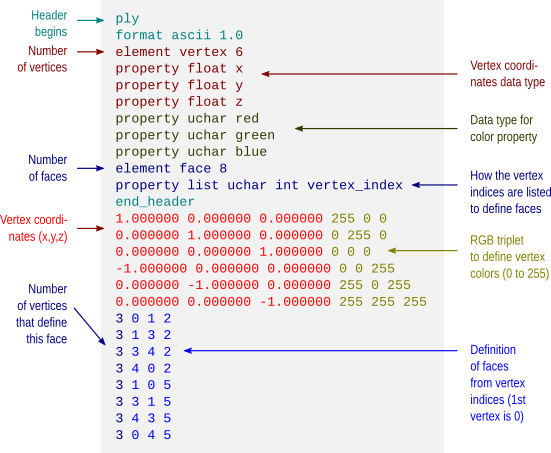
A solution is as follows: create a large file in the NTFS partition, install Linux inside this file, and boot the system from an USB flash drive. To discourage curiosity, the file can be encrypted. This article describes the steps to accomplish this task using openSUSE, but a similar strategy should work with any recent distribution.

Requirements

  • A computer with an NTFS partition, inside which you want to have Linux, without tampering with the actual Windows installation.
  • openSUSE installation DVD (tested with 12.1, and should work with other recent versions). Similar steps may work with other distributions.
  • USB flash drive which will be used to boot the Linux system and will also store the kernel. This flash drive must stay connected during all the time in which the system is on, therefore it is more convenient if it is physically small. See a picture below.
  • An external USB hard disk, to be used for a temporary installation that will be transferred to the file in the NTFS partition.

The procedure

Step 1: Plug the external hard disk and install openSUSE in it. Choose the desktop environment that suits you better (e.g. KDE/GNOME or other). It’s advisable to make this choice now, as it will save you time and effort, instead of leaving to add the graphical mode later. Leave /boot on its own partition as it will also facilitate steps later. Do not create a swap partition for this installation (ignore warnings that may appear because of this). Let’s call this as the system “E”, as it will reside temporarily on the External disk.

During the installation, install GRUB to the external disk itself, not to the internal drive (i.e., not /dev/sda), as you don’t want to tamper with the structure of internal hard drive or with the way as Windows boots. Before restarting the new system, if you changed the partitioning of the external disk, make sure that the partition that contains /boot has the “bootable” flag active (use fdisk to fix if needed).

Step 2: Make another install of openSUSE, this time to the flash drive. Again, put /boot on its own partition. Be generous with /boot, as it will accommodate 2 ramdisks and perhaps 2 or more kernels. Use at least 100MB. This installation can (and should) be the minimal, with no X (text-only). Let’s call this as system “F”, as it will reside in the USB Flash drive.

For a 16GB USB drive, a suggestion is:

  • 1st partition: 14GB, FAT or similar, to use as a general USB drive, nothing special.
  • 2nd partition: 1.8GB, ext4, to be mounted as as /, and where the system will reside.
  • 3rd partition: 0.2GB, ext4, to be mounted as /boot.

During the installation:

  • Like in the installation to the external hard disk, do not install GRUB to the internal drive, but to the USB memory stick.
  • For the list of software, install the ntfs-3g, ntfsprogs and cryptsetup. Install the man pages as well, as they may be useful.

Before booting the system F, make sure that the partition that contains /boot is bootable (use fdisk to fix if needed).

Step 3: Boot the system F, the flash drive. First task is to create the volume inside the NTFS filesystem, which will store the whole Linux system:

a) Create a key-file. No need for paranoia here, as the encryption is only to discourage any curious who sees these big files from Windows. Just a simple text file stored in the USB flash drive, separate from the encrypted volume:

echo SecretPassword | sha1sum > /root/key.txt

Note that in the command above, the password is not “SecretPassword”, but instead, the content of the file key.txt, as produced by the command sha1sum. This includes the space and dash (-) that are inside, as well as a newline character (invisible) at the end.

Do not store the keyfile in the NTFS partition. Put it, e.g., in the /root directory of the flash drive.

b) Mount the physical, internal hard drive that contains the NTFS partition:

mkdir -p /host
mount -t ntfs /dev/sda1 /host

c) Create a big file with random numbers in the NTFS partition. This will be the place where the full system will reside. For 100GB, use:

dd if=/dev/urandom of=/host/ntfsroot bs=2048 count=50000000

This will take several hours. You may want to leave it running overnight.

d) Mount it as a loop device:

losetup /dev/loop0 /host/ntfsroot

e) Initialize as a LUKS device:

cryptsetup luksFormat /dev/loop0 /root/key.txt

A message that any data on the device will irrevocably be deleted is shown. In this case, the device is the file full of random bits that we just created. So, confirm by typing ‘YES’ in capital letters.

f) Make a device-mapping:

cryptsetup luksOpen /dev/loop0 root --key-file /root/key.txt

This will create a /dev/mapper/root device, which is an unencrypted view of the content of the big file previously created. The /dev/loop0 is an encrypted view and is not meaningful for reading/writing.

g) Create the file system that later will host the root (i.e., /):

mkfs.ext4 -b 1024 /dev/mapper/root

The block size will be 1024. Smaller sizes will mean more free disk space for a given amount of stored data.

h) Repeat the steps b-g for what will be the swap partition (8GB in this example):

dd if=/dev/urandom of=/host/ntfspage bs=2048 count=4000000
losetup /dev/loop1 /host/ntfspage
cryptsetup luksFormat /dev/loop1 /root/key.txt
cryptsetup luksOpen /dev/loop1 swap --key-file /root/key.txt
mkswap /dev/mapper/swap

Step 4: [optional] Having made the initial configurations for the future / and swap, it’s now time to make a small modification of the initrd of the flash drive, so that it can boot from USB 3.0 if needed (even if the flash drive itself is 2.0, this step is still needed if you plan to plug it into an USB 3.0 port in the same computer):

a) Make a backup copy of the original initrd and update the symbolic link:

cd /boot
cp -p initrd-3.1.0-1.2-desktop initrd-3.1.0-1.2-opensuse
rm initrd
ln -s initrd-3.1.0-1.2-opensuse initrd

b) Edit the /etc/sysconfig/kernel and add the xhci-hcd module to the initial ramdisk:

INITRD_MODULES="xhci-hcd"

c) Run mkinitrd to create a new ramdisk.

cd /boot
mkinitrd

d) Rename it to something more representative:

mv /boot/initrd-3.1.0-1.2-desktop /boot/initrd-3.1.0-1.2-usbflash

The newly generated initrd will load the system that will be left in the flash drive, now with support for USB 3.0, and won’t be changed from now on.

Step 5: Restart the computer and boot into the system E (the external hard disk)

a) Edit the /etc/sysconfig/kernel and add these modules to the initial ramdisk:

INITRD_MODULES="xhci-hcd fuse loop dm-crypt aes cbc sha256"

Again, the xhci-hcd module is to allow booting the system from an USB 3.0 port (even if the flash drive is 2.0). If you don’t have USB 3.0 ports, this module can be omitted. The other modules are necessary to mount the NTFS partition, to mount files as a loopback devices, and to allow encryption/decryption using the respective algorithms and standards.

b) Run mkinitrd to create a new ramdisk.

cd /boot
mkinitrd

c) Make a copy of the newly created initrd to a place where it can be edited.

cp /boot/initrd-3.1.0-1.2-desktop /root/initrd-3.1.0-1.2-harddisk
mkdir /root/initrd-harddisk
cd /root/initrd-harddisk
cat ../initrd-3.1.0-1.2-harddisk | gunzip | cpio -id

d) Inside the initrd, edit the file boot/83-mount.sh (i.e. /root/initrd-harddisk/boot/83-mount.sh) and replace all its content by:

#!/bin/bash

# This will be the mountpoint of the NTFS partition
mkdir -p /host

# Mount the NTFS partition
ntfs-3g /dev/sda1 /host

# Mount the 100GB file as a loop device
losetup /dev/loop0 /host/ntfsroot

# Open the file for decryption (as a mapped device)
cryptsetup luksOpen /dev/loop0 root --key-file /key.txt

# Mount the ext4 filesystem on it as /root
mount -o rw,acl,user_xattr -t ext4 /dev/mapper/root /root

# Mount the 8GB file as a loop device
losetup /dev/loop1 /host/ntfspage

# Open the file for decryption (as a mapped device)
cryptsetup luksOpen /dev/loop1 swap --key-file /key.txt

e) Copy the losetup, cryptsetup, dmsetup and ntfs-3g executables to the initrd:

cp /sbin/losetup /sbin/cryptsetup /sbin/dmsetup /root/initrd-harddisk/sbin
cp /usr/bin/ntfs-3g /root/initrd-harddisk/bin

f) Copy also all the required libraries for these executables that may be missing (use ldd to discover which). There is certainly a way to script this, but to prepare and test the script will take as much time as to copy them manually. This has to be done just once.

g) Recreate the initrd:

cd /root/initrd-harddisk
find . | cpio -H newc -o | gzip -9 > ../initrd-3.1.0-1.2-harddisk

h) Copy the new initrd to the /boot partition of the USB flash drive, not to the /boot of the external hard disk. So, plug the USB drive and mount its boot partition:

mkdir -p /mnt/usbroot
mount -t ext4 /dev/sdX3 /mnt/usbboot
cp -p /root/initrd-3.1.0-1.2-harddisk /mnt/usbboot/

Step 6: Restart the system, now booting again into the system F (the USB flash drive):

a) Create two short scripts to mount and umount the encrypted filesystem. This will save time when you boot through the pendrive to do any maintenance on the installed system:

#!/bin/bash
mkdir -p /host
mount -t ntfs /dev/sda1 /host
losetup /dev/loop0 /host/ntfsroot
cryptsetup luksOpen /dev/loop0 root --key-file /root/key.txt
mkdir -p /mnt/ntfsroot
mount -t ext4 /dev/mapper/root /mnt/ntfsroot
#!/bin/bash
umount /mnt/ntfsroot
rmdir /mnt/ntfsroot
cryptsetup luksClose root
losetup -d /dev/loop0
umount /dev/sda1
rmdir /host

b) Execute the first, so that the file in the NTFS partition is mounted at /mnt/ntfsroot.

c) Mount the external disk partition that contains the / for the system E:

mkdir -p /mnt/hdroot
mount -t ext4 /dev/sdc2 /mnt/hdroot

d) Copy the whole system to the new location:

cp -rpv /mnt/hdroot/* /mnt/ntfsroot/

After this point, the external hard drive is no longer necessary. It can be unmounted and put aside.

e) Edit the /mnt/ntfsroot/etc/fstab to reflect the new changes:

/dev/mapper/swap    swap    swap    defaults          0  0
/dev/mapper/root    /       ext4    acl,user_xattr    1  1

Step 7: Modify GRUB to load the appropriate initrd and load the respective system. Open the /boot/grub/menu.lst and make it look something like this:

default 0
timeout 8

title openSUSE 12.1 -- Hard Disk
    root (hd0,2)
    kernel /vmlinuz-3.1.0-1.2-desktop splash=silent quiet showopts vga=0x317
    initrd /initrd-3.1.0-1.2-harddisk

title openSUSE 12.1 -- USB Flash Drive
    root (hd0,2)
    kernel /vmlinuz-3.1.0-1.2-desktop splash=silent quiet showopts vga=0x317
    initrd /initrd-3.1.0-1.2-usbflash

title Windows XP
    map (hd1) (hd0)
    map (hd0) (hd1)
    rootnoverify (hd1,0)
    makeactive
    chainloader +1

The only difference between the first and second entries is the initrd. In the first, the initrd will load the system that is inside the file in the NTFS partition, and which will contain the full graphical system. In the second, the initrd will load the simpler, text-only install on the USB flash drive.

Concluding remarks

We installed a modern, cutting edge Linux distribution inside a regular file in an NTFS partition. We did not modify any of the settings of Windows XP, neither did we partition the internal hard disk, nor tampered with the Windows registry or did anything that would violate any company rule. The boot loader, the kernel, and the initrd were left in an external device, the USB flash drive. When seen from Windows, only two inoffensive and unsuspicious files appear in the C:\. They contain the quiescent power of Linux.

Braindering with ASCII files

Binary file formats are faster to read and occupy less space for storage. However, when developing tools or when analysing data using non-standard methods, ascii files are easier to treat, and allow certain errors to be spotted immediately. Working with ascii files offer a number of advantages in these circumstances: the content of the files are human readable, meaning that there is no need for any special program other than perhaps a simple text editor, and can be manipulated easily with tools as sed or awk. It should be noted though, that while binary files require attention with respect to endianess and need some metadata to be correctly read, ascii need proper attention to end-of-line characters, that vary according to the operating system.

In articles to be posted soon I hope to share some tools to analyse and visualise brain imaging data. To use these tools, the files must be in ascii format. Each of these formats is discussed below and an example is given for a simple octahedron.

FreeSurfer surface (*.asc | suggested: *.srf)

FreeSurfer natively saves its surface files in binary form. The command mris_convert allows conversion to ascii format. The file extension is *.asc. This extension, however, is ambiguous with the curvature format (see below), reason for which a recommendation is to rename from *.asc to *.srf immediately after conversion.

The *.asc/*.srf format has a structure as described below. This format does not allow storing normals, colors, materials, multiple objects or textures. Just simple geometry.

FreeSurfer curvature (*.asc | suggested: *.dpv)

A curvature file contains a scalar value assigned to each vertex. This file format does not store the geometry of the surface and, in binary form, a curvature file simply contains one scalar per vertex. In ascii format, the vertex coordinates are also saved, but not how these vertices relate to define faces and the overall geometry.

Like with the FreeSurfer surface files, curvature files in ascii format also have the extension *.asc. To avoid confusion, it is suggested to rename from *.asc to *.dpv (data-per-vertex) immediately after conversion.

Facewise data (*.dpf)

This is not a native format from FreeSurfer, but a modification over the ascii curvature file described above. The file stores a scalar value per face, i.e. data-per-face (dpf) and, instead of saving vertex coordinates as with the *.dpv files, here the vertex indices that define the faces are saved. It is done like so because if both *.dpv and *.dpf files are present for a given geometric object, the object can be reconstructed with very little manipulation using simply awk. Currently there is no binary equivalent format.

VTK polygonal data (*.vtk)

A number of file formats have been developed over the years for use with the Visualization Toolkit (vtk). Some of these formats are now considered as “legacy” and are being phased out in favour of xml formats. Despite this, they are still used by a number of applications, such as fsl/first. The octahedron above in vtk polygonal data (polydata) format would have a structure as depicted below.

Wavefront Object (*.obj)

Wavefront Object files have a very simple structure, yet are powerful to allow definition of textures, normals and different materials. The format is supported by a variety of different graphic applications. The octahedron above would have a file structure as shown below.

The example does not show colors. However, it is possible to assign a material to each face, and materials contain their own color. These materials are typically stored in a separate file, a Materials Library, with extension *.mtl. An example for the same octahedron, both the object file and its associated materials library, is here: octa-color.obj and octa-color.mtl.


Many computer graphics software, however, limit the number of colors per object to a relatively small number, as 16 or 32. Blender, however, allows 32767 colors per object, a comfortable space for visualization of complex images, such as brain maps.

Stanford Polygon (*.ply)

The Stanford Polygon file allows not only the geometry to be stored, but also allow colours, transparency, confidence intervals and other properties to be assigned at each vertex. Again, the octahedron would have a file structure as:


This format also allows color attributes to be assigned to each vertex, as shown below.


The resulting object would then look like:

Batch conversion

Conversion between FreeSurfer formats can be done using mris_convert. A script to batch convert all FreeSurfer surface and curvature files from binary format to ascii is available here: subj2ascii. Before running, make sure FreeSurfer is correctly configured, that the variable SUBJECTS_DIR has been correctly set, and that you have writing permissions to this directory. Execute the script with no arguments to get usage information. The outputs (*.srf and *.dpv) are saved in a directory called ascii inside the directory of the subject. For many subjects, use a for-loop in the shell.

For more information

  • A description of the FreeSurfer file formats is available here.
  • A description of the different vtk (legacy and current) is available here.
  • Specification of the Wavefront obj format is here. Material library files are described here.
  • A description of the Stanford ply format is here.

Update — 28.May.2012: A script to convert from FreeSurfer .asc/.srf to .obj is here.
Update — 26.Jul.2013: This post was just updated to include examples of color formats.

Quickly inspect FreeSurfer cortical surfaces

To quickly inspect the surface reconstruction and parcellations produced by the cortical stream of FreeSurfer, rather than laboriously open each hemisphere at a time in tksurfer, an easier solution is to run a script that captures images, organise and present them all in a single html page that can be seen in any browser.

Before you start

Before you start, make sure you have:

  • FreeSurfer, any version released in the last 2 years. The procedure has been tested up to version 5.1.0.
  • ImageMagick, any recent version. For most Linux, ImageMagick can be installed directly from the distro’s repository. For Mac, it can be obtained with MacPorts or Fink.
  • The scripts takeshots, makehtml, shots_tksurfer.tcl, and shots_tkmedit.tcl. Put all these scripts into the same directory and make takeshots and makehtml executable.

Capturing the images

  1. Make sure recon-all finished for all your subjects. If there are no results, obviously there won’t be anything to inspect.
  2. Make sure the variable SUBJECTS_DIR is correctly set, pointing to the directory that contains the subjects, and that you have writing permissions to this directory.
  3. Prepare a text file containing a list of subjects, one per line, like this:
    subj001
    subj002
    ...
    subjNN
  4. Run the takeshots script. A typical usage is like this:
    ./takeshots -l listsubj.txt -m pial -m inflated -p aparc
    The options are:
    -l: List of subjects.
    -s: Additional subjects not in the list.
    -m: Surfaces to inspect (pial, inflated, white, sphere, etc).
    -p: Parcellations to inspect (aparc, aparc.a2005s, aparc.a2009s, etc).
    This script will create a subdirectory called ‘shots’ inside the directory of each subject, and will store a number of .tif files that are the different views of the cortical surfaces.
  5. Run the makehtml script. A typical usage is like this:
    ./makehtml -l listsubj.txt -m pial -m inflated -p aparc -d /path/to/html
    The options are identical to the previous command, with the addition of the option -d that lets you specify a directory where the html will be created. If this directory doesn’t exist, it will be created.

What you get

Open the file index.html in the directory specified in the previous step. There you’ll see all the surfaces of all the subjects, all in the same page, allowing you to quickly compare and have an idea of how good or bad they are. To see the name of the subject, hover the mouse on the corresponding image. Click on the image to see it larger. An example, using only pial and inflated surfaces, and the aparc parcellation, is here.

False Discovery Rate: Corrected & Adjusted P-values

Until mid-1990’s, control of the error rate under multiple testing was done, in general, using family-wise error rate (FWER). An example of this kind of correction is the Bonferroni correction. In an influential paper, Benjamini and Hochberg (1995) introduced the concept of false discovery rate (FDR) as a way to allow inference when many tests are being conducted. Differently than FWER, which controls the probability of committing a type I error for any of a family of tests, FDR allows the researcher to tolerate a certain number of tests to be incorrectly discovered. The word rate in the FDR is in fact a misnomer, as the FDR is the proportion of discoveries that are false among all discoveries, i.e., proportion of incorrect rejections among all rejections of the null hypothesis.

Benjamini and Hochberg’s FDR-controlling procedure

Consider testing N hypotheses, H_{1}, H_{2}, \ldots , H_{N} based on their respective p-values, p_{1}, p_{2}, \ldots , p_{N}. Consider that a fraction q 
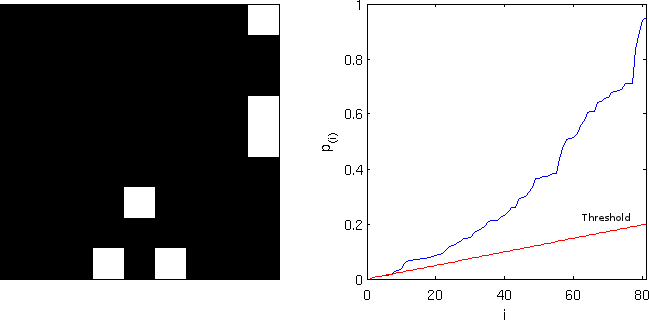
of discoveries are allowed (tolerated) to be false. Sort the p-values in ascending order, p_{(1)} \leq p_{(2)} \leq \ldots \leq p_{(N)} and denote H_{(i)} the hypothesis corresponding to p_{(i)}. Let k be the largest i for which p_{(i)} \leq \frac{i}{N}\frac{q}{c(N)}. Then reject all H_{(i)}, i=1, 2, \ldots , k. The constant c(N) is not in the original publication, and appeared in Benjamini and Yekutieli (2001) for cases in which independence cannot be ascertained. The possible choices for the constant are c(N)=1 or c(N)=\sum_{i=1}^{N} 1/i. The second is valid in any situation, whereas the first is valid for most situations, particularly where there are no negative correlations among tests. The B&H procedure has found many applications across different fields, including neuroimaging, as introduced by Genovese et al. (2002).

FDR correction

The procedure described above effectively defines a single number, a threshold, that can be used to declare tests as significant or not at the level q. One might, instead, be interested to know, for each original p-value, the minimum q level in which they would still be rejected. To find this out, define q_{(i)}=\frac{p_{(i)}N}{i}c(N). This formulation, however, has problems, as discussed next.

FDR adjustment

The problem with the FDR-correction is that q_{(i)} 
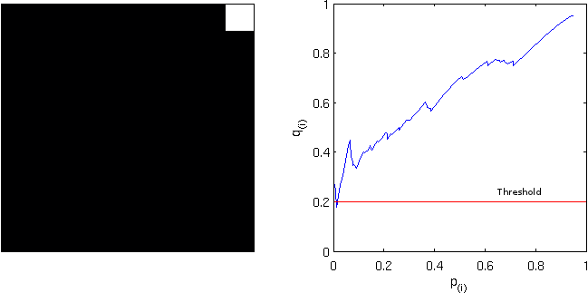
is not a monotonic function of p_{(i)}. This means that if someone uses any q_{(i)} to threshold the set of FDR-corrected values, the result is not the same as would be obtained by applying sequentially the B&H procedure for all these corresponding q levels.

To address this concern, Yekutieli and Benjamini (1999) introduced the FDR-adjustment, in which monotonicity is enforced, and which definition is compatible with the original FDR definition. Let q*_{(i)} 
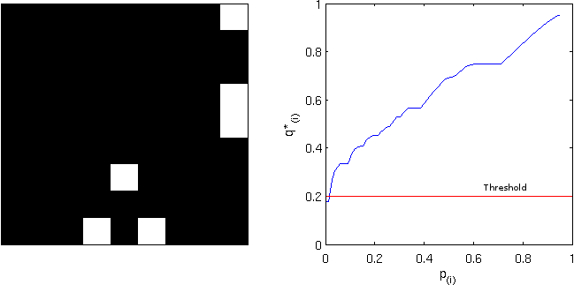
be the FDR-adjusted value for p_{(i)}. It’s value is the smallest q_{(k)}, k \geq i, where q_{(k)} is the FDR-corrected as defined above. That’s just it!

Example

Consider the image below, on the left, a square of 9×9 pixels containing each some t-statistic with some sparse, low magnitude signal added. On the right are the corresponding p-values, ranging approximately between 0-1:

Statistical maps

Statistic and p-values

colorscale

Using the B&H procedure to compute the threshold, with q=0.20
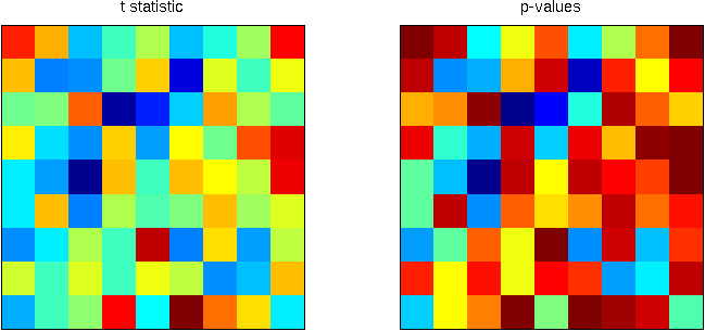
, and applying this threshold to the image rejects the null hypothesis in 6 pixels. On the right panel, the red line corresponds to the threshold. All p-values (in blue) below this line are declared significant.

FDR-threshold

FDR-threshold

Computing the FDR-corrected values at each pixel, and thresholding at the same q=0.20, however, does not produce the same results, and just 1 pixel is declared significant. Although conservative, the “correction” is far from the nominal false discovery rate and is not appropriate. Note on the right panel the lack of monotonicity.

FDR-corrected

FDR-corrected

Computing instead the FDR-adjusted values, and thresholding again at q=0.20 produces the same results as with the simpler FDR-threshold. The adjustment is, thus, more “correct” than the “corrected”. Observe, on the right panel, the monotonicity enforced.

FDR-adjusted

FDR-adjusted

Implementation

An implementation of the three styles of FDR for Octave/MATLAB is available here: fdr.m
SPM users will find a similar feature in the function spm_P_FDR.m.

References

Gaussian kernels: convert FWHM to sigma

When smoothing images and functions using Gaussian kernels, often we have to convert a given value for the full width at the half maximum (FWHM) to the standard deviation of the filter (sigma, \sigma). This happens because the implementation generally is in terms of sigma, while the FWHM is the more popular parameter in certain areas. The conversion is trivial, but it may well worth write it up here.

The probability density function (pdf) for the Gaussian distribution with mean \mu and standard deviation \sigma is:

f(x)=\frac{1}{\sigma\sqrt{2\pi}}e^{-\frac{(x-\mu)^2}{2\sigma^2}}

If the filter is centered at the origin, the mean is 0 and the FWHM is the distance between the -x_w and +x_w that produces the half of the peak. For the normal distribution, the mean is the same as the mode (peak) and we have then to find the x_w that will produce f(x_w) = f(\mu)/2:

\frac{1}{\sigma\sqrt{2\pi}}e^{-\frac{x_{w}^{2}}{2\sigma^2}} = \frac{1}{2} \frac{1}{\sigma\sqrt{2\pi}}

For \sigma \neq 0 and solving for x_w:

x_w = \pm \sqrt{2\sigma^2\ln 2}

The FWHM is +x_w - (-x_w)=2 x_w:

\text{FWHM}=2\sqrt{2\sigma^2\ln 2}=\sigma\sqrt{8\ln 2}

Which gives 2.35482004503 as the conversion factor, i.e., \text{FWHM} \approx 2.355\cdot \sigma.

Some software packages, such as SPM and FreeSurfer, interact with the user in terms of FWHM, whereas others, such as FSL, prefer \sigma. The relation above allows converting quickly between one and other representation.