Some image processing methods inherently smooth the images with an ideal filter, that is, a rectangular pulse. Comparing those methods with others that use a more typical Gaussian kernel can thus be challenging, as even if the full-width at half-maximum (FWHM) of the Gaussian filter is made equal to the width of the rectangular pulse, the resulting smoothnesses are not necessarily similar.
What would be the FWHM of a Gaussian filter that produces smoothness as similar as possible as that of a rectangular pulse of width ? This must depend only on the choice of the standard deviation of the Gaussian filter, which is the only parameter we can choose, versus the width of the ideal filter, which is also the only parameter that can be controlled (when it even can). If you ever wondered about this important question, here you will find the answer.
Note: This is the first time I use AI for an article (Claude 4.6, specifically). It certainly saved some time. I believe I am in good company in that.
Definitions: Consider first the 1D case. Let two real-valued functions each normalized to have unit area be:
1) A rectangular pulse of width :
2. A Gaussian centered at the origin with standard deviation :
We want to find the value of as a function of that minimizes the integral of squared difference between the two functions:
Solution: We start by expanding the integrand into 3 separate terms:
For , we substitute so
For , since on an interval of length and zero elsewhere, we have:
which does not depend on .
For , given that only on the interval , we have:
Substituting so that , and defining , thus mapping the integration limits to :
Noting that , we obtain:
Hence:
We need now to differentiate with respect to and set it to zero. The derivative of the first term is:
For the second term, using the chain rule with and , we have:
Setting :
and solving for :
Recalling we defined and solving for :
From a previous article, we know that the FWHM of a Gaussian filter can be expressed as .
Result for 1D: Hence, we have:
Which means that the FWHM of the Gaussian filter is approximately 0.8164965809277 times the width of the rectangular filter.
Result for 2D: If we repeat the process for the 2D case, in which the rectangular function forms a cylinder with radius and height so that the volume is equal to one, and seek the of the isotropic 2D Gaussian filter that has the minimal sum of squared differences in relation to the cylinder, after evaluating the double integrals, we find:
and thus, in the 2D case, we have a nice correspondence:
Result for 3D: If we do it again for the 3D case, changing now to a sphere of radius , and compute the of the corresponding isotropic 3D Gaussian, after evaluating the triple integrals, we find:
and thus, in the 3D case:
Which means that the FWHM of the Gaussian filter is approximately 1.264911064067352 times the width of the spherical filter.
Example: Suppose you did some image processing in a volumetric representation of the brain and that that involved averaging over a sphere with radius 30 mm. The width of the sphere is 60 mm. The FWHM of the closest Gaussian filter that yields similar degree of smoothing in the 3D case is approximately 75.8947 mm.
Download: A printer-friendly document with the derivations for 1D, 2D, and 3D cases, in the form of “exercises”, can be downloaded here.
This post describes a reimplementation of the method described by Caruyer et al. (2013). If you already know what this is about, you can skip the information below and simply download the code from GitHub: multishell.py. If you don’t know, a good place to start is Tuch et al. (2004).
Background
When we plan a magnetic resonance imaging protocol, we often have to balance what we would like to have in terms of quantity and quality of images, versus what can realistically be obtained within limited time slots (e.g., 30 minutes or 1 hour) while minimizing discomfort to the research participants, most of whom would rather not spend more than an hour in a somewhat uncomfortable MRI exam table. For diffusion weighted imaging, we want as many directions in q-space as possible, and that the directions are uniformly sampled across all possible directions, which help subsequent modelling of various diffusion parameters, fiber orientation and fiber crossings.
In practice, we need to establish a set of directions that uniformly covers the surface of a sphere. Presets available within the scanner workstation, provided by the manufacturer, are sometimes helpful but these are not entirely customizable. For example, for Siemens scanners, the number of directions can be selected as 6, 10, 12, 20, 30, 64, 128, or 256. But what if the number of directions for your experiment that makes best use of the time available is none of these? The problem becomes more complicated if there are multiple b-values (e.g., in a multishell acquisition or, e.g., with diffusion spectrum imaging). How to find the directions that uniformly sample all possible directions, without repetitions across shells, and while taking into account the multiple b-values?
Note that this is not simply a matter of finding random points uniformly distributed on the surface of a sphere. That could be done by simply generating independent Gaussian noise in the 3D space, then scaling the distance of each point to the center of the coordinate system to a certain radius, e.g., 1 (that is, treating each point as a vector and scaling it to unit norm). Instead, what we want are directions that are as far apart from each other as possible, so that the resulting image for each provides maximally unique information.
Moreover, having an arbitrary number of points equally separated on the surface of a sphere is impossible. Only five configurations exist, with at most 20 points; these configurations correspond to vertex locations of the five Platonic polyhedra. We need, therefore, to be content with values that are as spaced as possible on the surface, already knowing they can’t be all equally spaced.
Cost function
For just one b-value (one shell), a possible solution is to treat each direction as a charged particle in the surface of a sphere centered at the center of the coordinate system. The positions of the particles can then be established such that the electrostatic repulsion forces are minimized (Conturo et al., 1996; Jones et al., 1999). Caruyer et al. (2013) extended the idea to multiple b-values (multiple shells). Using the same notation as in the original paper, consider the repulsion force between particles represented by their positions (vectors) and (Equation 3 in the paper):
The above takes into account the direct repulsion between the two particles (first term, with a difference in the denominator) as well as repulsion between their antipodal representations (second term, with a sum in the denominator). Caruyer et al. (2013) then go on to propose the following cost functions for intra-shell and inter-shell electrostatic forces:
Intra-shell uniformity: Minimizing intra-shell electrostatic repulsion forces ensures that the points (directions) within each shell are evenly spread (Equation 2 if the paper):
where is the number of shells, and is the number of points (directions) on shell .
Inter-shell uniformity: Minimizing inter-shell electrostatic repulsion forces ensures that points across all shells, when projected onto a unit sphere, are evenly spread (Equation 4 in the paper):
where is the total number of points across all shells.
We have therefore two cost-functions that can be combined with a suitable factor that gives more or less weight for repulsions within- or between-shells:
under the constraint that all points need to lie on the surface of a sphere of radius 1.
Gradient
The gradient of the cost function in the Cartesian space is provided in Equation 7 of the paper:
where are the axes directions in the Cartesian coordinate system, i.e., , and where again the first term within brackets considers the repulsion forces of the particles themselves, whereas the second considers their antipodal representations.
Antipodal points
The inclusion of the antipodal representations of the points in the cost function is necessary otherwise whenever an even number of directions is considered, they would always lineup perfectly, pairwise, in antipodal sides of the sphere. Such configuration would not be optimal for diffusion imaging as the scanner would sample twice along the same direction and, despite opposite signs, result in the same diffusion weighted images, and thus provide repeated information (Jones et al., 1999). Consider, for example, a minimal case of only two directions: the best configuration (lowest repulsion force, lowest energy) is the one in which the two points are as far away from each other as possible, thus being on opposite sides of the sphere, and both ultimately leading to the same image. By including the antipodal points in the cost function (the second term in the equation for , as well as the corresponding term in the gradient function) as new charged particles, we avoid this problem: for the minimal case of two particles, the two directions will be orthogonal one to another, thus each one providing maximally unique information.
The alpha parameter
The weight parameter ranges between 0 and 1 and controls how much we want to emphasize intra-shell repulsion forces (greater , towards 1) or inter-shell repulsion forces (smaller , towards 0). While it may seem natural to choose = 0.50, that not necessarily yields optimal results. In the implementation provided here, the default is set as = 0.75, and the user can change its value until results are satisfactory.
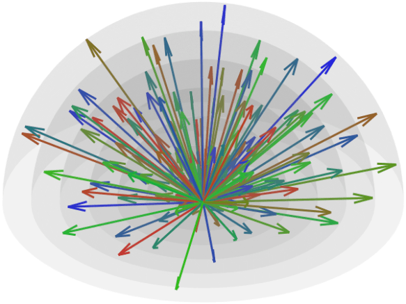
Effect of varying the parameter alpha for S = 2 shells and K = 100 directions (50 per shell). Low values of alpha cause the vectors not to be well spaced within shell, but well separated between shells; large values of alpha tend to have the opposite effect. Although alpha = 0.50 may seem a reasonable tradeoff, the best result seem to depend on the number of directions, shells, and the number of directions per shell. In the above example, among the 5 configurations, alpha = 0.75 appears to provide the most uniform coverage within and across shells. In the left column, the directions are represented as arrows, in the middle column, the directions are presented as blobs on the surface of each shell, and in the third column, the directions are reprojected to be shown in a single sphere (as if all shells had the same radius). The figure shows only one hemisphere for clarity, but approximately half of the directions shown are in fact in the opposite hemisphere. Click here for a larger figure.
Simultaneous optimization
For a number of desired directions, the best solution can be found by starting with random vectors in the unit sphere, spread them across shells, and allow them to move freely on each iteration on the surface of the sphere until the energy (repulsion force) is minimized, under the constraint that all directions lie on the unit sphere. Optimization can use the Nelder-Mead method (Jones et al., 1999), albeit the constraint would need to be imposed manually at each iteration, or SLS-QP (Caruyer et al., 2013). The implementation provided here uses SLS-QP from SciPy.
Incremental optimization
The original paper also discusses an alternative optimization scheme whereby only one new direction is added to an existing set, while retaining all previous ones fixed (page 1537 of the paper, 1st column, just before the Results section, and references therein). By iteratively estimating each new direction, one can obtain a quasi-optimal solution that has as main advantage the fact that, if scanning is interrupted before all images have been collected, the collected images are still nearly optimal for later processing. In the implementation provided here, the option to optimize incrementally is provided. A new direction is added to the shell that currently has the highest relative deficit of directions in relation to the desired final number of directions per shell. Although SLS-QP could be used, it is simpler to bypass the constraint by operating with spherical coordinates and using L-BFGS-B instead; this also allows faster reordering, as discussed next.
Optimal reordering of directions
While simultaneous optimization guarantees directions as spread as possible on the surface of each shell, and also when all shells are considered, incremental optimization ensures that informative data can be obtained if the imaging acquisition needs to be interrupted. In principle, you would have to choose between the two. Instead, in the implementation provided here, an option that combines of both schemes is provided: first, all directions are found via simultaneous optimization, then, while keeping the first direction fixed the second direction is the one which, among those already identified, that has the lowest repulsion force in relation to the first; the process is repeated for the third direction, finding the one, among those previously identified and not yet already selected, that has the lowest repulsion force in relation to the previous two; the process is iterated until all directions have been reordered. This can be used also with existing directions (i.e., without any new optimization). To use this feature, use the option –reorder.
In practice
The reimplementation described in this article is called multishell.py. It’s one single file that can be made executable and run as a command directly from the shell (e.g., from bash or zsh). Alternatively, it can be imported into your Python scripts, such that you can invoke the functions within it directly (e.g., the optimizer functions).
mpl_toolkits, specifically, the mplot3d toolkit, if you want to plot the directions as blobs (default) or rings
Assuming the file has been downloaded, made executable, and is in the current directory, then usage/syntax information is available with:
./multishell.py --help
File formats
In this reimplementation, the directions can be saved in files that can be imported directly by Siemens (*.dvs), General Electric (*.dat), or Philips scanners (*.txt). The directions can also be saved in FSL format (*.bvec/bval, also used by BIDS), in MRtrix3 format (*.b), or in the tabular format used by two earlier implementations provided by Emmanuel Caruyer (this and this). Conversion between any of these formats is also possible.
Some file formats require the specification of the b-values for each shell before they can be saved (e.g., Siemens, GE, FSL, MRtrix3). Some file formats require the specification of the maximum b-value so they can be correctly be read (e.g., Siemens, GE). The tabular formats used by Caruyer’s implementations do not specify b-values, only shell indices (they can start at 0 or 1 depending on the implementation). Hence, conversion from/to certain formats may require additional options, namely –bvalues and –bmax (more on this below).
Creating and saving a new scheme
The options –new and –save create and save a set of directions, respectively. Assuming that the multishell.py file has been downloaded, made executable, and is in the current directory, the options to create a new sampling scheme are:
where method can be simultaneous or incremental, K is the total number of directions, S is the number of shells, distr is how the directions should be distributed across shells (evenly, linearly, quadratically), and Ks is a list (provided between single quotes) of directions per shell. To save, use:
./multishell.py --save <prefix> <format> ...
where prefix is the prefix of the file(s) that will be created, and format is the format (siemens, ge, philips, fsl, mrtrix3, caruyer).
For example, say you want to specify a number of directions = 100, a number of shells = 3, that the number of directions should be spread across the shells linearly, that they should be optimized simultaneously to be optimally spaced, with weighting parameter = 0.75, and with b-values for each shell 1000, 2000, and 3000 s/mm2, then save the new scheme to a file for use in a Siemens scanner, then use:
Or say you want 4 shells, the first with 15 directions, the second with 29, the third with 47, and the fourth with 68 directions, that they should be optimized incrementally to allow optimal data use in case the acquisition is interrupted, that the b-values should be 800, 1600, 2400, and 3200 s/mm2, and want to save as a file for use in a GE scanner, use:
./multishell.py --new incremental '[15,29,47,68]' --bvalues '[800,1600,2400,3200]' --save myprefix ge
Or maybe you want as many shells as directions, with diffusion spectrum imaging (DSI) in mind:
Files with existing directions can be loaded for conversion, plotting, or manipulation with the option –load:
./multishell.py --load <filename> <format> ...
where filename is the name of the file to be loaded (with extension) and format is their format (siemens, ge, philips, fsl, mrtrix3, caruyer). For the FSL format, either the bvec or bval file can be specified, but both must exist.
Format conversions
Say you have a pair of bvec/bval files from data collected elsewhere, and want to use the same directions in a new acquisition in a Siemens scanner, then use:
In another example, suppose you have a set of directions from a Siemens scanner (which does not store actual b-values, just their relative magnitudes in relation to the maximum specified in the MRI parameter card), and want to use them in a Philips scanner (a format that stores the bvalues). When the sequence is run in the Siemens scanner, the bvalue is set as 2500 s/mm2. Then use:
Perhaps in the last conversion, you also wanted to reorder existing directions so that they allow optimal use of the data if the acquisition is interrupted. Then simply add the option –reorder:
The option –alpha can be used when reordering directions if you do not want to stay with the default.
Adding or removing b0
If your existing file includes acquisitions with b-values = 0 (i.e., without the application of diffusion-weighted gradients), you can remove them with the option –removeb0.
./multishell.py --removeb0 ...
You can also add some b-values = 0 at the beginning, intersperse them regularly throughout the acquisition, and/or add some to the end with the option –addb0. Say you want to add 5 b0 volumes at the beginning and 2 at the end:
./multishell.py --addb0 '[5,0,2]' ...
Or maybe you want a few, say 8, interspersed throughout the acquisition:
./multishell.py --addb0 '[5,8,2]' ...
For most formats, the directions associated with b-values = 0 are simply (0,0,0), but for Philips scanners, these need to be unique, so random directions are used instead. Also note that for Philips, the first b-value must always be 0, so with this format, regardless whether –addb0 is used or not, if the first direction does not have a b-value = 0 at the time the file is saved, one will be added at the beginning.
Plotting
Basic plotting of the directions is available with the option –plot. When invoking from the shell, you can specify a file format for saving (e.g., pdf, eps, svg, png); four plots will be produced: with and without reprojecting all shells to unit sphere, and with the directions represented as arrows or as blobs.
./multishell.py --plot svg ...
If instead of a file format you provide the keyword interactive, it will open the plots in a window to allow interactive visualization, manipulation of the figure, and saving.
./multishell.py --plot interactive ...
Since antipodal points are included in the cost function, all directions can, for visualization purposes, be represented in only one hemisphere. However, that is only for display; the vectors themselves have equal likelihood of being in one hemisphere or another, thus covering the whole surface of the sphere.
Order of arguments and of operations
The order the arguments are provided is not relevant. If the same argument is repeated, it is the last one that counts. Inside the program, the operations happen in the following order:
The options –new or –load are executed, thus either creating or loading a set of directions.
If a file in a format that does not include b-values was loaded, or if a new set of directions was just created, the option –bvalues is parsed, thus defining the b-values for each shell.
The option –reorder is executed if provided, thus optimally reordering the directions.
The option –removeb0 is executed if provided, thus removing directions that have been assigned a b-value = 0.
The option –addb0 is executed if provided, thus adding b-values = 0 and corresponding directions.
The option –save is executed if provided, thus saving the set of directions to a file in the specified format.
The option –plot is executed if provided, thus showing the directions (interactive mode) or saved to a file in the specified format (png, pdf, svg, eps, and various others supported by matplotlib).
Integration with your Python code
If you prefer not to use the function from the system shell and prefer instead to call it from your Python code, you can do that too. Place the file multishell.py where you can import it, then call the functions as needed. A simple example is:
import multishell as ms
import numpy as np

# Number of directions
K = 120

# Number of shells
S = 3

# b-values of each shell
blist = [1000, 2000, 3000]

# Distribute the number of directions across shells
Ks = ms.directions_per_shell(K, S, 'quadratically')

# Simultaneous optimization of all directions
vectors, shells = ms.simultaneous_optimization(Ks, alpha=0.75, maxiter=100)

# Optimally reorder the directions
vectors, shells, idx = ms.optimal_reordering(vectors, shells)

# b-values for each corresponding direction
bvalues = np.array(blist)[shells[:,0]][:,None]

# Save in FSL format
fileprefix = 'mydirs'
ms.write_fsl(fileprefix, vectors, bvalues)

# Plot
ms.plot_directions(vectors, bvalues=bvalues, colorby='acquisition', style='quiver', reproject=False)
Why a new implementation?
Two helpful implementations provided by Caruyer are available. One is a webtool that allows up to 5 shells and up to 500 directions be downloaded after estimation via incremental optimization, but it doesn’t allow specification of the weighting parameter , and only saves the directions in a tabular format that requires further manipulation before it can be used in the scanner. The other is a Python version that uses simultaneous optimization and provides finer control, but the shells are indexed differently from the webtool, and doesn’t include incremental optimization; it also doesn’t save directly in a format that can be used in common scanners. It allows plotting, but in my system figures appear incorrectly cropped. Conversion tools for Siemens and GE are available, but they require additional installation of packages for format changes that are relatively simple. For the webtool, there is always a risk that it may no longer be available in the future; as a concrete example, when the directions were downloaded for use in the Human Connectome Project (Sotiropoulos et al., 2013), it was located at a different address, hosted by the INRIA, now no longer accessible (broken link). Additionally, I could not understand Figure 2 in the original paper (compare with the figures above), and I had to implement it to understand what was going on. Finally, an all-in-one tool was much needed by our group as we plan on projects and need to find best use of scanner time. As this new implementation is helpful to us, it is hoped it will be helpful to you as well.
References
The most important reference is the original paper by Caruyer and colleagues, and which should be cited in case you use this reimplementation in your research:
Marek, Tervo-Clemmens et al. (2022) suggest that we need much larger sample sizes to investigate associations between common variability in brain structure or function and cognition or psychiatric symptomatology. That is true under the assumption that such associations, for complex, multifactorial cognitive or psychiatric phenotypes, and characteristics accessible with existing imaging methods, exist.
Unfortunately, the evidence provided seems to suggest the absence of such effects. In their article, Figure 2 shows overlap only for the distribution of effects, with peaks virtually at zero for three major studies, but no evidence for overlap of localized effects; Supplementary Figure 17 shows near-perfect correlation for average connectivity, but not for connectivity in relation to complex phenotypes. In Linke et al. (2021), we showed evidence that similar clinical presentations can emerge from disparate changes in brain connectivity, suggesting substantial diversity in the presentation of the underlying biological substrate, even for the same behavioral measurements.
It is possible that the aspects of human behavior that we consider relevant, and which guide our cognitive and clinical phenotyping, do not manifest themselves as measurable entities using available brain imaging methods. Merely increasing sample size with such phenotypes can only ensure statistically significant results for trivial, negligible effects, which may still fail to replicate. More investment on the development of techniques to probe yet unexplored aspects of the brain tissue, in vivo, and non-invasively, are more likely to be fruitful, without prejudice to the collection of large samples. The same holds for cognitive and clinical phenotypes, which need to be reliable, even if only indirectly mapped into aspects of human behavior.
Anderson M. Winkler, Daniel S. Pine, Julia O. Linke
Very often we find ourselves handling large matrices and, for multiple different reasons, may want or need to reduce the dimensionality of the data by retaining the most relevant principal components. A question that arises then is how many such principal components should be retained? That is, what are the principal components that provide information that can be distinguished from variability that is indistinguishable from random noise?
One simple heuristic method is the scree plot (Cattell, 1966): one computes the singular values of the matrix, plots them in descending order, and visually looks for some kind of “elbow” (or the starting point of the “scree”) to be used as a threshold. Those singular vectors (principal components) that have corresponding singular values larger than that threshold are retained, otherwise discarded. Unfortunately, the scree test is too subjective, and worse, many realistic problems can produce matrices that have multiple such “elbows”.
Many other methods to help select the number of principal components to retain exist. Some, for example, are based on information theory, or on probabilistic formulations, or on hard thresholds related the size of the matrix or the (explained) variance from the data. In this article, the little known Wachter method (Wachter, 1976) is presented.
Let be a matrix of random values with zero mean and variance . The density of the bulk spectrum of the singular values , , , of is:
and a point mass at the origin if , where , , and (Bai, 1999). This is the Marčenko and Pastur (1967) distribution. The cumulative distribution function (cdf) can be obtained by integration, i.e., . MATLAB/Octave functions that compute the cdf and its inverse are here: mpcdf.m and mpinv.m.
If we know the probability of finding a singular value or larger for a random matrix, we have the means to judge whether that is sufficiently large to be considered interesting enough for its corresponding singular vector (principal component) to be retained. Simply computing the p-value, however, is not enough, because the distribution makes no reference to the position of the sorted singular values. A different procedure needs be considered.
The core idea of the Wachter method is to use a QQ plot of the observed singular values versus the quantiles obtained from the inverse cdf of the Marčenko–Pastur distribution, and use eventual deviations from the identity line to help finding the threshold that separates the “good” from the “unnecessary” principal components. That is, plot the eigenvalues versus the quantiles . Deviations from the identity line are evidence for excess variance not expected from random variables alone.
The function wachter.m computes the singular values from a given observed matrix , the expected singular values should be a random matrix, as well as the p-values for each singular value in either case. The observed and expected singular values can be used to built a QQ-plot. The p-values can be used for a comparison, e.g., via the logarithm of their ratio. For example:
% For reproducibility, reset the random number generator.
% Use "rand" instead of "rng" to ensure compatibility with old versions.
rand('seed',0);

% Simulate data. See Gavish and Donoho (2014) for this example.
X = diag([1.7 2.5 zeros(1,98)]) + randn(100)*sqrt(.01);

% Compute the expected and observed singular values,
% as well as the respective cumulative probabilities (p-values).
% See the help of wachter.m for syntax.
[Exp,Obs,Pexp,Pobs] = wachter(X,[],false,true);

% Log of the ratio between observed and expected p-values.
% Large values are evidence for "good" components.
P_ratio = -log10(Pobs./Pexp);

% Plot the spectrum.
subplot(1,2,1);
plot(Obs,'x:');
title('Singular values');
xlabel('index (k)');

% Construct the QQ-plot.
subplot(1,2,2);
qqplot(Exp,Obs);
title('QQ plot');
The result is:
In this example, two of the singular values can be considered “good”, and should be retained. The others can, according to this criterion, be dropped.
The function can take into account nuisance variables (provided in the 2nd argument), including intercept (for mean-centering), allows normalization of columns to unit variance, and can operate on p-values (upper tail from the density function) or on the cumulative probabilities. See the help text inside the function for usage information.
Wachter KW. Probability plotting points for principal components.In: Proceedings of the Ninth Interface Symposium on Computer Science and Statistics. Harvard University and Massachussetts Institute of Technology: Prindle, Weber & Schmidt; 1976. p. 299–308.
The image at the top is of the Drei Zinnen, in the Italian Alps during the Summer, in which a steep slope scattered with small stones (scree) is visible. Photo by Heinz Melion from Pixabay.
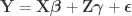
Doing a permutation test with the general linear model (GLM) in the presence of nuisance variables can be challenging. Let the model be:
where is a matrix of observed variables, is a matrix of predictors of interest, is a matrix of covariates (of no interest), and is a matrix of the same size as with the residuals.
Because the interest is in testing the relationship between and , in principle it would be these that would need be permuted, but doing so also breaks the relationship with , which would be undesirable. Over the years, many methods have been proposed. A review can be found in Winkler et al. (2014); other previous work include the papers by Anderson and Legendre (1999) and Anderson and Robinson (2001).
One of these various methods is the one published in Freedman and Lane (1983), which consists of permuting data that has been residualised with respect to the covariates, then estimated covariate effects added back, then the full model fitted again. The procedure can be performed through the following steps:
Regress against the full model that contains both the effects of interest and the nuisance variables, i.e., . Use the estimated parameters to compute the statistic of interest, and call this statistic .
Regress against a reduced model that contains only the covariates, i.e. , obtaining estimated parameters and estimated residuals .
Compute a set of permuted data . This is done by pre-multiplying the residuals from the reduced model produced in the previous step, , by a permutation matrix, , then adding back the estimated nuisance effects, i.e. .
Regress the permuted data against the full model, i.e.
Use the estimated to compute the statistic of interest. Call this statistic .
Repeat the Steps 2-4 many times to build the reference distribution of under the null hypothesis of no association between and .
Count how many times was found to be equal to or larger than , and divide the count by the number of permutations; the result is the p-value.
Steps 1-4 can be written concisely as:
where is a permutation matrix (for the -th permutation, is the hat matrix due to the covariates, and is the residual forming matrix; the superscript symbol represents a matrix pseudo-inverse.
[…] add the nuisance variables back in Step 3 is not strictly necessary, and the model can be expressed simply as , implying that the permutations can actually be performed just by permuting the rows of the residual-forming matrix .
However, in the paper we do not offer any proof of this important result, that allows algorithmic acceleration. Here we remedy that. Let’s start with two brief lemmata:
Lemma 1: The product of a hat matrix and its corresponding residual-forming matrix is zero, that is, .
Lemma 2 (Frisch–Waugh–Lovell theorem): Given a GLM expressed as , we can estimate from an equivalent GLM written as .
To see why, remember that multiplying both sides of an equation by the same factor does not change it (least squares solutions may change; transformations using Lemma 2 below do not act on the fitted model). Let’s start from:
Then remove the parentheses:
Since :
and that :
Since :
where .
Main result
Now we are ready for the main result. The Freedman-Lane model is:
Per Lemma 2, it can be rewritten as:
Dropping the parenthesis:
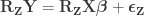
Per Lemma 1:
What is left has the same form as the result of Lemma 2. Thus, reversing it, we obtain the final result:
Hence, the hat matrix cancels out, meaning that it is not necessary. Results are the same both ways.
We often think of statistics as a way to summarize large amounts of data. For example, we can collect data from thousands of subjects, and extract a single number that tells something about these subjects. The well known German tank problem shows that, in a certain way, statistics can also be used for the opposite: using incomplete data and a few reasonable assumptions (or real knowledge), statistics provides way to estimate information that offer a panoramic view of all the data. Historical problems are interesting on their own. Yet, it is not always that we see so clearly consequential historical events at the time they happen — like now.
In the Second World War, as in any other war, information could be more valuable than anything else. Intelligence reports (such as from spies) would feed the Allies with information about the industrial capacity of Nazi Germany, including details about things such as the number of tanks produced. This kind of information can have far reaching impact and not only determine the outcome of a battle, but also if a battle would even even happen or with what preparations, as the prospect of finding a militarily superior opponent is often a great deterrent.
Sometimes, German tanks, as the well known Panzer, could be captured and carefully inspected. Among the details noted were the serial number printed in various pieces, such as chassis, gearboxes, and the serial numbers of the moulds used to produce the wheels. With the serial number of even a single chassis, for example one can estimate the total number of tanks produced; knowing the serial number of a single wheel mould allows the estimation of the total number of moulds, and thus, how many wheels can be produced in a certain amount of time. But how?
If serial numbers are indeed serial, e.g., , growing uniformly and without gaps, and we see a tank that has a serial number , then clearly at least tanks must have been produced. But could we have a better guess?
Let’s start by reversing the problem: suppose we knew . In that case, what would be the average value of the serial numbers of all tanks? The average for uniformly distributed data like this would be , that is, the average of the first and last serial numbers.
Now, say we have only one sighting of a tank, and that has serial number . Then our best guess for the average serial number is itself, as we have no additional information. Thus, with , our guess would be (that is, reorganizing the terms of the previous equation for ). Note that, for one sighting, this formula guarantees that is larger or equal than , which makes sense: we cannot have an estimate for that is smaller than the serial number itself.
What if we had not just one, but multiple sightings? Call the number of sightings . The mean is now , for ordered serial numbers . Clearly, we can’t use the same formula, because if is much smaller than (say, because we have seen many small serial numbers, but just a handful of larger ones), could incorrectly be estimated as less than , which makes no sense. At least tanks must exist.
While incorrect for , the above formula gives invaluable insight: it shows that for such uniformly distributed data, approximately half of the tanks have serial number above , the other half below . Extending the idea, and still under the assumption that the serial numbers are uniform, we can conclude that the number of tanks below the lowest serial number (which is ) must be approximately the same as the (unknown) number of tanks above the highest serial number . So, a next better estimate could be to use .
We can still do better, though. Since we have sightings, we can estimate what is the average interval between sightings, i.e., . As it is based on all sightings, this gives a better estimate of the spacing between the serial numbers than the single sighting . The result can be added to . The final estimate then becomes .
To make this concrete, say we saw tanks numbered . Then our best guess would be .
At the end of the war, estimates obtained using the above method proved remarkably accurate, much more so than information provided by spies and other intelligence reports.
Let’s now see a similar example that is contemporary to us. Take the current pandemic caused by a novel coronavirus. The World Health Organization stated officially, in 14th January 2020, when there were 41 cases officially reported in China, that there was no evidence for human-to-human transmission. Yet, when the first 3 cases outside China were confirmed in 16th January 2020, epidemiologists at the Imperial College London were quick to find out that the WHO statement must have not been true. Rather, the real number of cases was likely well above 1700.
Preliminary investigations conducted by the Chinese authorities have found no clear evidence of human-to-human transmission of the novel #coronavirus (2019-nCoV) identified in #Wuhan, #China🇨🇳. pic.twitter.com/Fnl5P877VG
How did they make that estimate? The key insight was the realisation that only a small number of people in any major city travels internationally, particularly in such a short time span like that given by the time until the onset of symptoms for this kind of respiratory disease. If one can estimate prevalence among those who travelled, that would be a good approximation to the prevalence among those who live in the city, assuming that those who travel are an unbiased sample of the population.
Following this idea, we have: , that is, the number of cases among those who travelled () divided by the total number of people who travelled () is expected to be approximately the same as the number of cases among those who stayed () divided by the total number of people who stayed (live) in the city ().
The number of people served by the international airport of Wuhan is about 19 million (the size of the Wuhan metropolitan area), and the average daily number of outbound international passengers in previous years was 3301 for that time of the year (a figure publicly known, from IATA). Unfortunately, little was known outside China about the time taken between exposure to the virus and the onset of symptoms. The researchers then resorted to a proxy: the time known for the related severe respiratory disorder known as MERS, also caused by a coronavirus, which is about 10 days. Thus, we can estimate people travelling out, and staying in the city. The number of known international cases was at the time . Hence:
cases
So, using remarkably simple maths, simpler even than in our WWII German tank example, the scientists estimated that the number of actual cases in the city of Wuhan was likely far above the official figure of 41 cases. The researchers were careful to indicate that, should the probability of travelling be higher among those exposed, the number of actual cases could be smaller. The converse is true: should travellers be wealthier (thus less likely to be exposed to a possible zoonosis as initially reported), the number of actual cases could be higher.
Importantly, it is not at all likely that 1700 people would have contracted such a zoonosis from wild animals in a dense urban area like Wuhan, hence human-to-human transmission must had been occurring. Eventually the WHO confirmed human-to-human transmission on 19th January 2020. Two days later, Chinese authorities began locking down and sealing off Wuhan, thus putting into place a plan to curb the transmission.
To find out more about the original problem of the number of tanks, and also for other methods of estimation for the same problem, a good start is this article. Also invaluable, for various estimation problems related to the fast dissemination of the novel coronavirus, are all the reports by the epidemiology team at the Imperial College London, which can be found here.
In canonical correlation analysis (CCA; Hotelling, 1936), the absolute value of a correlation is not always that helpful. For example, large canonical correlations may arise simply due to a large number of variables being investigated using a relatively small sample size; high correlations may arise simply because there are too many opportunities for finding mixtures in both sides that are highly correlated one with another.
Motivated by this perceived difficulty in the interpretation of results, Stewart and Love (1968) proposed the computation of what has been termed a redundancy index. It works as follows.
Let and be two sets of variables over which CCA is computed. We find canonical coefficients and , such that the canonical variables and have maximal, diagonal correlation structure; this diagonal contains the ordered canonical correlations.
Now that CCA has been computed, we can find the correlations between the original variables and the canonical coefficients. Let and be such correlations, which are termed canonical loadings or structure coefficients. Now compute the mean square for each of the columns of and . These represent the variance extracted by the corresponding canonical variable. That is:
Variance extracted by canonical variable :
Variance extracted by canonical variable :
These quantities represent the mean variance extracted from the original variables by each of the canonical variables (in each side).
Compute now the proportion of variance of one canonical variable (say, ) explained by the corresponding canonical variable in the other side (say, ). This is given simply by , the usual coefficient of determination.
The redundancy index for each canonical variable is then the product of and for the left side of CCA, and the product of and for the right side. That is, the index is not symmetric. It measures the proportion of variance in one of the two set of variables explained by the correlation between the -th pair of canonical variables.
The sum of the redundancies for all canonical variables in one side or another forms a global redundancy metric, which indicates the proportion of the variance in a given side explained by the variance in the other.
This global redundancy can be scaled to unity, such that the redundancies for each of the canonical variables in a give side can be interpreted as the proportion of total redundancy.
If you follow the original paper by Stewart and Love (1968), and are column III of Table 2, the redundancy of each canonical variable for each side corresponds to column IV, and the proportion of total redundancy is in column V.
Another reference on the same topic that is worth looking is Miller (1981). In it, the author discusses that redundancy is somewhere in between CCA itself (fully symmetric) and multiple regression (fully asymmetric).
PALM — Pemutation Analysis of Linear Models — uses either MATLAB or Octave behind the scenes. It can be executed from within either of these environments, or from the shell, in which case either of these is invoked, depending on how PALM was configured.
For users who do not want or cannot spend thousands of dollars in MATLAB licenses, Octave comes for free, and offers quite much the same benefits. However, for Octave, some functionalities in PALM require version 4.4.1 or higher. However, stable Linux distributions such as Red Hat Enterprise Linux and related (such as CentOS and Scientific Linux) still offer only 3.8.2 in the official repositories at the time of this writing, leaving the user with the task of finding an unofficial package or compiling from the source. The latter task, however, can be daunting: Octave is notoriously difficult to compile, with a myriad of dependencies.
A much simpler approach is to use Flatpak or Snappy. These are systems for distribution of Linux applications. Snappy is sponsored by Canonical (that maintains Ubuntu), whereas Flatpak appears to be the preferred tool for Fedora and openSUSE. Using either system is quite simple, and here the focus is on Flatpak.
To have a working installation of Octave, all that needs be done is:
Only the installation of Flatpak needs be done as root. Once it has been installed, repositories and applications (such as Octave, among many others) can be installed at the user level. These can also be installed and made available system-wide (if run as root).
Configuring PALM
From version alpha117 onwards, the executable file ‘palm’ (not to be confused with ‘palm.m’) will include a variable named “OCTAVEBIN”, which specifies how Octave should be called. Change it from the default:
OCTAVEBIN=/usr/bin/octave
so that it invokes the version installed with Flatpak:
OCTAVEBIN="/usr/bin/flatpak run org.octave.Octave"
After making the above edits, it should be possible to run PALM directly from the system shell using the version installed via Flatpak. Alternatively, it should also be possible to invoke Octave (as in step 4 above), then use the command “addpath” to specify the location of palm.m, and then call PALM from the Octave prompt.
Octave packages
Handling of packages when Octave is installed via Flatpak is the same as usual, that is, via the command ‘pkg’ run from within Octave. More details here.
NiDB is a light, powerful, and simple to use neuroimaging database. One of its main strengths is that it was developed using a stack of stable and proven technologies: Linux, Apache, MySQL/MariaDB, PHP, and Perl. None of these technologies are new, and the fact that they have been around for so many years means that there is a lot of documentation and literature available, as well as a myriad of libraries (for PHP and Perl) that can do virtually anything. Although both PHP and Perl have received some degree of criticism (not unreasonably), and in some cases are being replaced by tools such as Node.js and Python, the volume of information about them means it is easy to find solutions when problems appear.
This article covers installation steps for either CentOS or RHEL 7, but similar steps should work with other distributions since the overall strategy is the same. By separating apart each of the steps, as opposed to doing all the configuration and installation as a single script, it becomes easier to adapt to different systems, and to identify and correct problems that may arise due to local particularities. The steps below are derived from the scripts setup-centos7.sh and setup-ubuntu16.sh, that are available in the NiDB repository, but here these will be ignored. Note that the instructions below are not “official”; for the latter, consult the NiDB documentation. The intent of this article is to facilitate the process and mitigate some frustration you may feel if trying to do it all by yourself. Also, by looking at the installation steps, you should be able to have a broad overview of the pieces that constitute database.
1) Begin with a fresh install.
If installing CentOS from the minimal DVD, choose a “Minimal Install” and leave to add the desktop in the next step.
2) Update the system.
This is a good time to install the most recent updates and patches, and reboot if the updates include a new kernel:
yum update
/sbin/reboot
3) Have a graphical mode.
While not strictly necessary, having a graphical interface for a web-based application will be handy. Install your favourite desktop, and a VNC server if you intend to manage the system remotely. For a lightweight desktop, consider MATE:
First add the EPEL repository. Depending on what you already have configured, use either:
For VNC, there are various options available. Consider, for example, TurboVNC.
4) Define some environment variables to be used later.
These will help when entering the commands later.
# Directory where NiDB will be installed
NIDBROOT=/nidb

# Directory of the webpages and PHP files:
WWWROOT=/var/www/html

# Linux username under which NiDB will run:
NIDBUSER=nidb

# MySQL/MariaDB root password:
MYSQLROOTPASS=[YOUR_PASSWORD_HERE]

# MySQL/MariaDB username that will have access to the database, and associated password:
MYSQLUSER=nidb
MYSQLPASS=[YOUR_PASSWORD_HERE]
These variables are only used during the installation, and all the steps here are done as root. Considering clearing your shell history at the end, so as not to have your passwords stored there.
5) Create an account for the user under which NiDB will run.
This is the user that will run the processes related to the database. It is not necessary that this user has administrative privileges on the system, and from a security perspective, it is better if not.
useradd -m ${NIDBUSER}
passwd ${NIDBUSER} # choose a sensible password
6) Install and configure Apache.
Add the repository for a more recent version, then install:
yum install httpd
Configure it to run as the ${NIDBUSER} user:
sed -i "s/User apache/User ${NIDBUSER}/" /etc/httpd/conf/httpd.conf
sed -i "s/Group apache/Group ${NIDBUSER}/" /etc/httpd/conf/httpd.conf
Pay attention to the questions on the root password and set it here to what was chosen in the ${MYSQLROOTPASS} variable. Make sure your database is secure.
Install also various Perl packages from CPAN. The first time you run cpan, various configuration questions will be asked; it is safe to accept default answers for all:
Disabling SELinux is not strictly necessary provided that you ensure that all processes related to NiDB (webserver, database server), and all its files, belong to the same user, nidb, and that file access policies are set correctly. In any case, you may feel this is useful so as to stop receiving too many irrelevant warnings during the installation. You can enable it again later.
sed -i 's/^SELINUX=.*/SELINUX=disabled/g' /etc/selinux/config
setenforce 0
Note that enabling or disabling SELinux requires a reboot to take effect (it is not sufficient to simply restart a daemon; there is not one in fact).
11) Install FSL.
FSL functions are used by various internal scripts. After the installation, make sure the environment variable FSLDIR exists and points to the correct location (typically /usr/local/fsl, but can be different if you installed it elsewhere). This variable is used below when defining the crontab jobs.
FSLDIR=/usr/local/fsl
12) Download and install the NiDB files.
The official Github repository is https://github.com/gbook/nidb. However, I have made a fork with a couple of changes that better adapt to the system I am working with. You can probably go with either way.
First, create the nidb user in MySQL/MariaDB. This is the only user (other than root) that will be able to do anything in the database:
mysql -uroot -p${MYSQLROOTPASS} -e "CREATE USER '${MYSQLUSER}'@'%' IDENTIFIED BY '${MYSQLPASS}'; GRANT ALL PRIVILEGES ON *.* TO '${MYSQLUSER}'@'%';"
Now create the NiDB database proper:
cd ${NIDBROOT}/install/setup
mysql -uroot -p${MYSQLROOTPASS} -e "CREATE DATABASE IF NOT EXISTS nidb; GRANT ALL ON *.* TO 'root'@'localhost' IDENTIFIED BY '${MYSQLROOTPASS}'; FLUSH PRIVILEGES;"
mysql -uroot -p${MYSQLROOTPASS} nidb < nidb.sql
mysql -uroot -p${MYSQLROOTPASS} nidb < nidb-data.sql
14) Setup cron jobs.
These jobs will take care of various automated input/output tasks.
The main configuration file, ${NIDBROOT}/programs/nidb.cfg, should be edited to reflect your paths, usernames, and passwords. It is this file that will contain the admin password for accessing NiDB. Use the ${NIDBROOT}/programs/nidb.cfg.sample as an example.
Once you have logged in as admin, you can also edit this file again in the database interface, in the menu Admin -> NiDB Settings.
16) (Optional) Install a MySQL/MariaDB frontend.
It will likely increase your productivity when doing maintenance to have a friendly frontend for MySQL/MariaDB. Two popular choices are phpMyAdmin (web-based) and Oracle MySQL Workbench.
You should by now have a working installation of NiDB, accessible from your web-browser at http://localhost. There are additional pieces you may consider configuring, such as a listener in one of your server ports to bring DICOMs from the scanner in automatically as the images are collected, and also other changes to the database schema and web interface. Now you have a starting point.
References
For more information on NiDB, see these two papers:
There are various ways one could estimate morphometric parameters of the cortex, such as its thickness, area, and volume. For example, it is possible to use voxelwise partial volume effects using volume-based representations of the brain, such as in voxel-based morphometry (VBM), in which estimates per voxel become available. Volume-based representations also allow for estimates of thickness, as suggested, for example, by Hutton et al. (2004), or from a surface representation of the cortex, in which it can be measured as a form of distance between the mesh that represents the pia mater (the pial surface) and the mesh that represents the interface between gray and white matter (the white surface).
Here we focus on the surface-based representation as that offers advantages over volume-based representations (Van Essen et al., 1998). Software such as FreeSurfer uses magnetic resonance images to initially construct the white surface. Once that surface has been produced, a copy of it can be offset outwards until tissue contrast in the magnetic resonance image is maximal, which indicates the location of the pial surface. This procedure ensures that both white and pial surfaces have the same topology, with each face and each vertex of the white surface having their matching pair in the pial. This convenience facilitates the computations indicated below.
Cortical surface area
For a triangular face of the surface representation, with vertex coordinates , , and , the area is , where , , represents the cross product, and the bars represent the vector norm. Even though such area per face (i.e., facewise) can be used in subsequent steps, most software packages can only deal with values assigned to each vertex (i.e., vertexwise). Conversion from facewise to vertexwise is achieved by assigning to each vertex one-third of the sum of the areas of all faces that meet at that vertex (Winkler et al., 2012).
Cortical thickness
The thickness at each vertex is computed as the average of two distances (Fischl and Dale, 2000; Greve and Fischl, 2018): the first is the distance from each white surface vertex to their corresponding closest point on the pial surface (not necessarily at a pial vertex); the second is the distance from the corresponding pial vertex to the closest point on the white surface (again, not necessarily at a vertex). Other methods are possible, however, see table below (adapted from Lerch and Evans, 2005):
If the area of either of these surfaces is known, or if the area of a mid-surface, i.e., the surface running half-distance between pial and white surfaces is known, an estimate of the volume can be obtained by multiplying, at each vertex, area by thickness. This procedure is still problematic in that it underestimates the volume of tissue that is external to the convexity of the surface, and overestimates volume that is internal to it; both cases are undesirable, and cannot be solved by merely resorting to using an intermediate surface as the mid-surface.
Figure 1: A diagram in two dimensions of the problem of measuring the cortical volume. If volume is computed using the product method (a), considerable amount of tissue is left unmeasured in the gyri, or measured repeatedly in sulci. The problem is minimised, but not solved, with the use of the mid-surface. In the analytic method (b), vertex coordinates are used to compute the volume of tissue between matching faces of white and pial surfaces, leaving no tissue under- or over-represented.
Analytic method
In Winkler et al. (2018) we propose a different approach to measure volume. Instead of computing the product of thickness and area, we note that any pair of matching faces can be used to define an irregular polyhedron, of which all six coordinates are known from the surface geometry. This polyhedron is an oblique truncated triangular pyramid, which can be perfectly divided into three irregular tetrahedra, which do not overlap, nor leave gaps.
Figure 2: A 3D diagram with the proposed solution to measure the cortical volume. In the surface representation, the cortex is limited internally by the white and externally by the pial surface (a). These two surfaces have matching vertices that can be used to delineate an oblique truncated triangular pyramid (b) and (c). The six vertices of this pyramid can be used to define three tetrahedra, the volumes of which are computed analytically (d).
From the coordinates of the vertices of these tetrahedra, their volumes can be computed analytically, then added together, viz.:
For a given face in the white surface, and its corresponding face in the pial surface, define an oblique truncated triangular pyramid.
Split this truncated pyramid into three tetrahedra, defined as:
For each such tetrahedra, let , , and represent its four vertices in terms of coordinates . Compute the volume as , where , , , the symbol represents the cross product, represents the dot product, and the bars represent the vector norm.
No error other than what is intrinsic to the placement of these surfaces is introduced. The resulting volume can be assigned to each vertex in a similar way as conversion from facewise area to vertexwise area. The above method is the default in FreeSurfer 6.0.0.
Is volume at all useful?
Given that volume of the cortex is, ultimately, determined by area and thickness, and these are known to be influenced in general by different factors (Panizzon et al, 2009; Winkler et al, 2010), why would anyone bother in even measuring volume? The answer is that not all factors that can affect the cortex will affect exclusively thickness or area. For example, an infectious process, or the development of a tumor, have potential to affect both. Volume is a way to assess the effects of such non-specific factors on the cortex. However, even in that case there are better alternatives available, namely, the non-parametric combination (NPC) of thickness and area. This use of NPC will be discussed in a future post here in the blog.

 the repulsion force between particles represented by their positions (vectors)
  and
and  (Equation 3 in the paper):

 is the number of shells, and
  is the number of points (directions) on shell
  .
.
 is the total number of points across all shells.
 in the Cartesian space is provided in Equation 7 of the paper:
 are the axes directions in the Cartesian coordinate system, i.e.,
  , and where again the first term within brackets considers the repulsion forces of the particles themselves, whereas the second considers their antipodal representations.
 , as well as the corresponding term in the gradient function) as new charged particles, we avoid this problem: for the minimal case of two particles, the two directions will be orthogonal one to another, thus each one providing maximally unique information.
 ranges between 0 and 1 and controls how much we want to emphasize intra-shell repulsion forces (greater
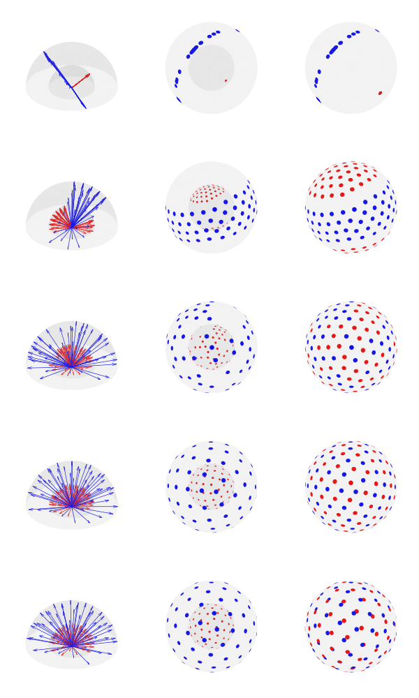
 of desired directions, the best solution can be found by starting with random vectors in the unit sphere, spread them across
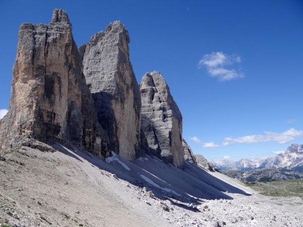
 be a
be a  matrix of random values with zero mean and variance
  . The density of the bulk spectrum of the singular values
  ,
,  ,
,  , of
, of  is:
is: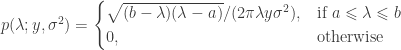
 at the origin if
  , where
  ,
,  , and
, and  (Bai, 1999). This is the Marčenko and Pastur (1967) distribution. The cumulative distribution function (cdf) can be obtained by integration, i.e.,
 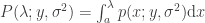 .
.  or larger for a random matrix, we have the means to judge whether that
  of the sorted singular values. A different procedure needs be considered.
 versus the quantiles
  . Deviations from the identity line are evidence for excess variance not expected from random variables alone.
 is a matrix of observed variables,
  is a matrix of covariates (of no interest), and
  is a matrix of the same size as
  to compute the statistic of interest, and call this statistic
  .
. , obtaining estimated parameters
  and estimated residuals
  .
. . This is done by pre-multiplying the residuals from the reduced model produced in the previous step,
  , then adding back the estimated nuisance effects, i.e.
 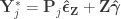 .
.
 to compute the statistic of interest. Call this statistic
  .
. under the null hypothesis of no association between
 is a permutation matrix (for the
  -th permutation,
  is the
  is the residual forming matrix; the superscript symbol
  represents a
 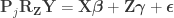 , implying that the permutations can actually be performed just by permuting the rows of the residual-forming matrix
  .
. .
. since
since  from an equivalent GLM written as
  .
.


 :
:
 :
:
 .
.


 cancels out, meaning that it is not necessary. Results are the same both ways.
 , growing uniformly and without gaps, and we see a tank that has a serial number
  . In that case, what would be the average value of the serial numbers of all
  , that is, the average of the first and last serial numbers.
 , our guess would be
  (that is, reorganizing the terms of the previous equation for
  ). Note that, for one sighting, this formula guarantees that
  , for ordered serial numbers
  . Clearly, we can’t use the same formula, because if
  (say, because we have seen many small serial numbers, but just a handful of larger ones),
  , the above formula gives invaluable insight: it shows that for such uniformly distributed data, approximately half of the tanks have serial number above
  (which is
  ) must be approximately the same as the (unknown) number of tanks above the highest serial number
  .
. . As it is based on all
  .
. . Then our best guess would be
  .
. , that is, the number of cases among those who travelled (
 ) divided by the total number of people who travelled (
 ) is expected to be approximately the same as the number of cases among those who stayed (
 ) divided by the total number of people who stayed (live) in the city (
 ).
). people travelling out, and
  staying in the city. The number of known international cases was at the time
  . Hence:
 cases
cases and
and  be two sets of variables over which CCA is computed. We find canonical coefficients
  and
and  ,
,  such that the canonical variables
  and
and  have maximal, diagonal correlation structure; this diagonal contains the ordered canonical correlations
  .
. and
and  be such correlations, which are termed canonical loadings or structure coefficients. Now compute the mean square for each of the columns of
  and
and  . These represent the variance extracted by the corresponding canonical variable. That is:
 :
: 
 :
: 
 , the usual coefficient of determination.
 and
and  and
and 

 of the surface representation, with vertex coordinates
 ![\mathbf{a}=[x_A \; y_A \; z_A]'](https://s0.wp.com/latex.php?latex=%5Cmathbf%7Ba%7D%3D%5Bx_A+%5C%3B+y_A+%5C%3B+z_A%5D%27&bg=ffffff&fg=333333&s=0&c=20201002) ,
, ![\mathbf{b}=[x_B \; y_B \; z_B]'](https://s0.wp.com/latex.php?latex=%5Cmathbf%7Bb%7D%3D%5Bx_B+%5C%3B+y_B+%5C%3B+z_B%5D%27&bg=ffffff&fg=333333&s=0&c=20201002) , and
, and ![\mathbf{c}=[x_C \; y_C \; z_C]'](https://s0.wp.com/latex.php?latex=%5Cmathbf%7Bc%7D%3D%5Bx_C+%5C%3B+y_C+%5C%3B+z_C%5D%27&bg=ffffff&fg=333333&s=0&c=20201002) , the area is
, the area is  , where
  ,
,  ,
,  represents the cross product, and the bars
  represent the vector norm. Even though such area per face (i.e., facewise) can be used in subsequent steps, most software packages can only deal with values assigned to each vertex (i.e., vertexwise). Conversion from facewise to vertexwise is achieved by assigning to each vertex one-third of the sum of the areas of all faces that meet at that vertex (

 in the white surface, and its corresponding face
  in the pial surface, define an oblique truncated triangular pyramid.
 ,
,  ,
,  and
and  represent its four vertices in terms of coordinates
 ![[x\;y\;z]'](https://s0.wp.com/latex.php?latex=%5Bx%5C%3By%5C%3Bz%5D%27&bg=ffffff&fg=333333&s=0&c=20201002) . Compute the volume as
. Compute the volume as  , where
  ,
,  ,
,  , the symbol
  represents the dot product, and the bars