Normality tests I: Brief overview

Before the fast computers era, it was difficult to test how valid certain statistical methods were. Even in the 1970’s and 1980’s, when computers were already available at Universities and even at home, certain matrix operations were limited by hardware constraints. We are now at a much more comfortable position to analyse how these methods perform. One area where (nowadays) simple computer runs can be illuminating is with respect to normality tests. Tests to evaluate normality or a specific distribution, frequentist approaches can be broadly divided into two categories:

Tests based on comparison (“best fit”) with a given distribution, often specified in terms of its cumulative distribution funtion (cdf). Examples are the Kolmogorov-Smirnov test, the Lilliefors test, the Anderson-Darling test, the Cramér-von Mises criterion, as well as the Shapiro-Wilk and Shapiro-Francia tests.
Tests based on descriptive statistics of the sample. Examples are the skewness test, the kurtosis test, the D’Agostino-Pearson omnibus test, the Jarque-Bera test.

In this article I’ll briefly review six well-known normality tests: (1) the test based on skewness, (2) the test based on kurtosis, (3) the D’Agostino-Pearson omnibus test, (4) the Shapiro-Wilk test, (5) the Shapiro-Francia test, and (6) the Jarque-Bera test. In a subsequent article, I’ll analyse the analytical p-value approximations for these tests, and in a third article, I’ll provide Monte Carlo critical values for each of them.

Skewness test

The skewness of the sample data can be converted to an useful score to evaluate normality with the following transformation (D’Agostino, 1970):

Compute the sample skewness $\sqrt{b_1} = m_3/m_2^{3/2}$ , where $m_k=\sum_i (X_i-\bar X)^k/n$ is the k-th moment, $\bar X=\sum_i X_i/n$ is the sample mean, and $n$ is the sample size.
Compute:
$Y = \sqrt{b_1}\left(\frac{(n+1)(n+3)}{6(n+2)}\right)^{1/2}$
$\beta_2(\sqrt{b_1}) = \frac{3(n^2+27n-70)(n+1)(n+3)}{(n-2)(n+5)(n+7)(n+9)}$
$W^2 = -1+(2(\beta_2(\sqrt{b_1})-1))^{1/2}$
$\delta = 1/\sqrt{\ln W}$
$\alpha = (2/(W^2-1))^{1/2}$
Compute:
$Z(\sqrt{b_1}) = \delta \ln(Y/\alpha + ((Y/\alpha)^2+1)^{1/2})$

The $Z(\sqrt{b_1})$ is the test statistic and it is approximately normally distributed under the null hypothesis that the population data follows a normal distribution.

Kurtosis test

Like the test based on skewness, the test based on kurtosis needs that the sample kurtosis is calculated, then transformed, and finally converted to a p-value. The steps are (Anscombe & Glynn, 1983):

Compute the sample kurtosis $b_2=m_4/m_2^2$ , where $m_k=\sum_i (X_i-\bar X)^k/n$ is the k-th moment, $\bar X=\sum_i X_i/n$ is the sample mean, and $n$ is the sample size.
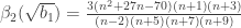
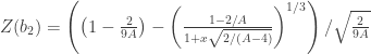
Compute:
$\mathsf{E}\{b_2\} = 3(n-1)/(n+1)$
$\mathsf{var}\{b_2\} = \frac{24n(n-2)(n-3)}{(n+1)^2(n+3)(n+5)}$
$x = (b_2-\mathsf{E}\{b_2\})/\sqrt{\mathsf{var}\{b_2\}}$
$\sqrt{\beta_1(b_2)}=\frac{6(n^2-5n+2)}{(n+7)(n+9)}\sqrt{\frac{6(n+3)(n+5)}{n(n-2)(n-3)}}$
$A = 6+\frac{8}{\sqrt{\beta_1(b_2)}}\left(\frac{2}{\sqrt{\beta_1(b_2)}}+\sqrt{1+\frac{4}{\beta_1(b_2)}}\right)$ , where $\mathsf{E}\{\cdot\}$ and $\mathsf{var}\{\cdot\}$ represent respectively the expected value and the variance.
Compute:
$Z(b_2) = \left(\left(1-\frac{2}{9A}\right)-\left(\frac{1-2/A}{1+x\sqrt{2/(A-4)}}\right)^{1/3}\right)/\sqrt{\frac{2}{9A}}$

The $Z(b_2)$ is the test statistic and is considered approximately normally distributed under the null hypothesis that the population data follows a normal distribution.

D’Agostino-Pearson omnibus test

The skewness and kurtosis tests can be combined to produce a single, global, “omnibus” statistic. This global test has been proposed by D’Agostino and Pearson (1973) and its statistic is simply $K^2=(Z(\sqrt{b_1}))^2 + (Z(b_2))^2$ . In other words, simply square the statistics from the skewness and kurtosis tests and sum them together. The distribution of the $K^2$ statistic is approximately a $\chi^2$ distribution with two degrees of freedom under the null hypothesis that the sample was drawn from a population with normally distributed values. The skewness, kurtosis and the D’Agostino-Pearson tests have been collectively reviewed and discussed in D’Agostino et al. (1990).

A matlab/Octave implementation of the D’Agostino-Pearson test is available here: daptest.m.

Jarque-Bera test

In a certain regard, this test, introduced by Jarque & Bera (1980) and later discussed in more detail in Jarque & Bera (1987), could also be called an “omnibus” test, that combines skewness and kurtosis into a single statistic. The test statistic is given by $\text{\textsc{lm}}= n\left(\frac{(\sqrt{b_1})^2}{6} + \frac{(b_2-3)^2}{24}\right)$ . The $\text{\textsc{lm}}$ is asymptotically distributed as a $\chi^2$ distribution with two degrees of freedom under the null hypothesis that the sample was drawn from a population with normally distributed values.

A matlab/Octave implementation of the Jarque-Bera test is available here: jbtest.m.

Shapiro-Wilk test

The Shapiro & Wilk (1965) test depends on the covariance matrix between the order statistics of the observations. Values for this covariance matrix have been laboriously tabulated for small samples (Sahan & Greenberg,1956) and algorithms have been developed (Davis & Stephens, 1978; Royston, 1982). In an effort to produce equivalents, yet computationally affordable results, it has been suggested to use approximations. The description here follow the approximation suggested by Royston (1992).

Sort the data in ascending order.
Compute the sample mean $\bar X=\sum_i X_i/n$ , where $n$ is the sample size.
Compute the Blom scores (Blom, 1958) as $\tilde m_i = \Phi^{-1}\{(i-3/8)/(n+1/4)\}$ , where $i$ is the rank order and $\Phi^{-1}\{\cdot\}$ represents the inverse normal cdf.
Compute a set of weights $c_i = \tilde m_i \sqrt{(\mathbf{\tilde m}'\mathbf{\tilde m})}$ . These weights are the same used in the Shapiro-Francia test (see below).
Compute $\tilde a_n= - 2.706056u^5 + 4.434685u^4 - 2.071190u^3 - 0.147981u^2 + 0.221157u + c_n$ , where $u=n^{-1/2}$ . If $n>5$ , compute also $\tilde a_{n-1}= -3.582633u^4 + 5.682633u^4 -1.752461u^3 -0.293762u^2 + 0.042981u + c_{n-1}$ .
Compute $\phi = (\mathbf{\tilde m}'\mathbf{\tilde m} - 2\tilde m_n^2)/(1-2\tilde a_n^2)$ if $n \leq 5$ or $\phi = (\mathbf{\tilde m}'\mathbf{\tilde m} - 2\tilde m_n^2 - 2\tilde m_{n-1}^2)/(1-2\tilde a_n^2-2\tilde a_{n-1}^2)$ otherwise.
Compute the remaining $\tilde a_i = \phi^{-1/2} \tilde m_i$ for $i=2, \ldots ,n-1$ if $n \leq 5$ or $i=3,\ldots ,n-2$ if $n>5$ .
Compute the test statistic $W=\left(\sum_i \tilde a_i X_i \right)^2 / \sum_i (X_i-\bar X)^2$ .

Once the test statistic $W$ has been produced, it can be approximated through a function $g(W)$ to a normal distribution with mean $\mu$ and standard deviation $\sigma$ (Royston, 1993). For sample sizes between 4 and 11 (inclusive), $g(W)=-\ln(\gamma-\ln(1-W))$ , where $\gamma=0.459n-2.273$ . For sample sizes equal to or larger than 12, $g(W)=\ln(1-W)$ .

For $4 \leq n \leq 11$ , the parameters of the statistic transformed (normalized) by $g(W)$ are given by $\mu=-0.0006714n^3 + 0.025054n^2 -0.39978n + 0.5440$ and $\sigma=\mathsf{exp}\{-0.0020322n^3+ 0.062767n^2 -0.77857n + 1.3822\}$ . For $n \geq 12$ , $\mu = 0.0038915u^3 -0.083751u^2 -0.31082u -1.5851$ and $\sigma = \mathsf{exp}\{0.0030302u^2 -0.082676u -0.4803\}$ , where $u = \ln(n)$ .

A $Z$ statistic can then be produced trivially by $(g(W)-\mu)/\sigma$ , and the p-values can be obtained from the normal cdf.

A matlab/Octave implementation of the Shapiro-Wilk test is available here: swtest.m.

Shapiro-Francia test

The test was proposed by Shapiro & Francia (1972) as a simplification of the Shapiro-Wilk test. The simplification consisted in replacing the covariance matrix of the order statistics by the identity matrix. The test is generally considered asymptotically equivalent to the Shapiro-Wilk test for large and independent samples. To apply the test, the steps are (Royston, 1993):

Sort the data in ascending order.
Compute the sample mean $\bar X=\sum_i X_i/n$ , where $n$ is the sample size.
Compute the Blom scores (Blom, 1958) as $\tilde m_i = \Phi^{-1}\{(i-3/8)/(n+1/4)\}$ , where $i$ is the rank order and $\Phi^{-1}\{\cdot\}$ represents the inverse normal cumulative distribution function (cdf).
Compute a set of weights $c_i = \tilde m_i \sqrt{(\mathbf{\tilde m}'\mathbf{\tilde m})}$ .
Compute the test statistic $W'=\left(\sum_i c_i X_i \right)^2 / \sum_i (X_i-\bar X)^2$ .

Similarly as for the Shapiro-Wilk test, once the test statistic $W'$ has been produced, it can be approximated through a function $g(W')=\ln(1-W')$ to a normal distribution with mean $\mu$ and standard deviation $\sigma$ (Royston, 1993). The parameters of the statistic transformed (normalized) by $g(W')$ are given by $\mu=1.0521u - 1.2725$ , where $u = \ln(\ln(n))-\ln(n)$ and $\sigma=-0.26758v+1.030$ , where $v = \ln(\ln(n))+2/\ln(n)$ . These approximations are valid for samples between 5 and 5000 at least.

References

- Anscombe FJ, Glynn WJ. Distribution of the Kurtosis Statistic b 2 for Normal Samples. Biometrika. 1983; 70(1):227-34.
- Blom G. Statistical Estimates and Transformed Beta-Variables. New York, NY. John Wiley & Sons, 1958.
- DʼAgostino RB. Transformation to Normality of the Null Distribution of g1. Biometrika. 1970; 57(3):679-81.
- DʼAgostino RB, Belanger A, DʼAgostino Jr RB. A Suggestion for Using Powerful and Informative Tests of Normality. The American Statistician. 1990; 44(4):316-21.
- DʼAgostino R, Pearson ES. Tests for Departure from Normality. Empirical Results for the Distributions of b 2 and √b 1. Biometrika. 1973; 60(3):613-22.
- Davis C, Stephens M. Approximating the Covariance Matrix of Normal Order Statistics. Applied Statistics. 1978; 27(2):206-212.
- Jarque CM, Bera AK. A Test for Normality of Observations and Regression Residuals. International Statistical Review/Revue Internationale de Statistique. 1987; 55(2):163–172.
- Jarque CM, Bera AK. Efficient tests for normality, homoscedasticity and serial independence of regression residuals. Economics Letters. 1980; 6(3):255-259.
- Royston P. Approximating the Shapiro-Wilk W-test for non-normality. Statistics and Computing. 1992; 2(3):117-119.
- Royston P. A Toolkit for Testing for Non-Normality in Complete and Censored Samples. The Statistician. 1993; 42(1):37.
- Royston JP. Algorithm AS 177: Expected normal order statistics (exact and approximate). Journal of the Royal Statistical Society. Series C (Applied Statistics). 1982; 31(2):161–165.
- Sarhan AE, Greenberg BG. Estimation of location and scale parameters by order statistics from singly and doubly censored samples. The Annals of Mathematical Statistics. 1956; 27(2):427–451.
- Shapiro SS, Wilk MB. An analysis of variance test for normality (complete samples). Biometrika. 1965; 52(3-4):591-611.
- Shapiro SS, Francia R. An approximate analysis of variance test for normality. Journal of the American Statistical Association. 1972; 67(337):215–216.
Pingback: Normality tests II: Asymptotic approximations « Brainder.
Pingback: Singapore Government Securities Yields: A Multi-Factor Heath, Jarrow And Morton Model | OptionFN
Pingback: Carlin cap Lessons From The U.S. Treasury Market, 1962-2019 – Premier league
After computing the k2 How would I know if I am going to reject the null hypothesis or not in using D’Agostino-Pearson omnibus test?
Hi Nash,
The D’Agostino-Pearson K^2 statistic follows a Chi^2 distribution with 2 degrees of freedom, from which p-values can be computed.
Hope this helps!
All the best,
Anderson
Pingback: A 10 Factor Heath, Jarrow and Morton Stochastic Volatility Model for the U.S. Treasury Yield Curve, Using Daily Data from January 1, 1962 through December 31, 2020 - Kamakura Corporation
Pingback: A 10 Factor Heath, Jarrow, and Morton Stochastic Volatility Model for the U.S. Treasury Yield Curve, Using Daily Data from January 1, 1962 through June 30, 2021 - Kamakura Corporation
Pingback: A 7-Factor Heath, Jarrow, and Morton Stochastic Volatility Model for the Government of Canada Yield Curve, Using Daily Data from January 2, 2001 through August 31, 2021 - Kamakura Corporation
Pingback: An 11-Factor Heath, Jarrow, and Morton Stochastic Volatility Model for the Government of Russia Yield Curve, Using Daily Data from January 4, 2003 through August 31, 2021 - Kamakura Corporation
Pingback: A 15-Factor Heath, Jarrow, and Morton Stochastic Volatility Model for the German Bund Yield Curve, Using Daily Data from August 7, 1997 through September 30, 2021 - Kamakura Corporation
Pingback: A 10-Factor Heath, Jarrow, and Morton Stochastic Volatility Model for the U.S. Treasury Yield Curve, Using Daily Data from January 1, 1962 through September 30, 2021 - Kamakura Corporation