Some image processing methods inherently smooth the images with an ideal filter, that is, a rectangular pulse. Comparing those methods with others that use a more typical Gaussian kernel can thus be challenging, as even if the full-width at half-maximum (FWHM) of the Gaussian filter is made equal to the width of the rectangular pulse, the resulting smoothnesses are not necessarily similar.
What would be the FWHM of a Gaussian filter that produces smoothness as similar as possible as that of a rectangular pulse of width ? This must depend only on the choice of the standard deviation of the Gaussian filter, which is the only parameter we can choose, versus the width of the ideal filter, which is also the only parameter that can be controlled (when it even can). If you ever wondered about this important question, here you will find the answer.
Note: This is the first time I use AI for an article (Claude 4.6, specifically). It certainly saved some time. I believe I am in good company in that.
Definitions: Consider first the 1D case. Let two real-valued functions each normalized to have unit area be:
1) A rectangular pulse of width :
2. A Gaussian centered at the origin with standard deviation :
We want to find the value of as a function of that minimizes the integral of squared difference between the two functions:
Solution: We start by expanding the integrand into 3 separate terms:
For , we substitute so
For , since on an interval of length and zero elsewhere, we have:
which does not depend on .
For , given that only on the interval , we have:
Substituting so that , and defining , thus mapping the integration limits to :
Noting that , we obtain:
Hence:
We need now to differentiate with respect to and set it to zero. The derivative of the first term is:
For the second term, using the chain rule with and , we have:
Setting :
and solving for :
Recalling we defined and solving for :
From a previous article, we know that the FWHM of a Gaussian filter can be expressed as .
Result for 1D: Hence, we have:
Which means that the FWHM of the Gaussian filter is approximately 0.8164965809277 times the width of the rectangular filter.
Result for 2D: If we repeat the process for the 2D case, in which the rectangular function forms a cylinder with radius and height so that the volume is equal to one, and seek the of the isotropic 2D Gaussian filter that has the minimal sum of squared differences in relation to the cylinder, after evaluating the double integrals, we find:
and thus, in the 2D case, we have a nice correspondence:
Result for 3D: If we do it again for the 3D case, changing now to a sphere of radius , and compute the of the corresponding isotropic 3D Gaussian, after evaluating the triple integrals, we find:
and thus, in the 3D case:
Which means that the FWHM of the Gaussian filter is approximately 1.264911064067352 times the width of the spherical filter.
Example: Suppose you did some image processing in a volumetric representation of the brain and that that involved averaging over a sphere with radius 30 mm. The width of the sphere is 60 mm. The FWHM of the closest Gaussian filter that yields similar degree of smoothing in the 3D case is approximately 75.8947 mm.
Download: A printer-friendly document with the derivations for 1D, 2D, and 3D cases, in the form of “exercises”, can be downloaded here.
This post describes a reimplementation of the method described by Caruyer et al. (2013). If you already know what this is about, you can skip the information below and simply download the code from GitHub: multishell.py. If you don’t know, a good place to start is Tuch et al. (2004).
Background
When we plan a magnetic resonance imaging protocol, we often have to balance what we would like to have in terms of quantity and quality of images, versus what can realistically be obtained within limited time slots (e.g., 30 minutes or 1 hour) while minimizing discomfort to the research participants, most of whom would rather not spend more than an hour in a somewhat uncomfortable MRI exam table. For diffusion weighted imaging, we want as many directions in q-space as possible, and that the directions are uniformly sampled across all possible directions, which help subsequent modelling of various diffusion parameters, fiber orientation and fiber crossings.
In practice, we need to establish a set of directions that uniformly covers the surface of a sphere. Presets available within the scanner workstation, provided by the manufacturer, are sometimes helpful but these are not entirely customizable. For example, for Siemens scanners, the number of directions can be selected as 6, 10, 12, 20, 30, 64, 128, or 256. But what if the number of directions for your experiment that makes best use of the time available is none of these? The problem becomes more complicated if there are multiple b-values (e.g., in a multishell acquisition or, e.g., with diffusion spectrum imaging). How to find the directions that uniformly sample all possible directions, without repetitions across shells, and while taking into account the multiple b-values?
Note that this is not simply a matter of finding random points uniformly distributed on the surface of a sphere. That could be done by simply generating independent Gaussian noise in the 3D space, then scaling the distance of each point to the center of the coordinate system to a certain radius, e.g., 1 (that is, treating each point as a vector and scaling it to unit norm). Instead, what we want are directions that are as far apart from each other as possible, so that the resulting image for each provides maximally unique information.
Moreover, having an arbitrary number of points equally separated on the surface of a sphere is impossible. Only five configurations exist, with at most 20 points; these configurations correspond to vertex locations of the five Platonic polyhedra. We need, therefore, to be content with values that are as spaced as possible on the surface, already knowing they can’t be all equally spaced.
Cost function
For just one b-value (one shell), a possible solution is to treat each direction as a charged particle in the surface of a sphere centered at the center of the coordinate system. The positions of the particles can then be established such that the electrostatic repulsion forces are minimized (Conturo et al., 1996; Jones et al., 1999). Caruyer et al. (2013) extended the idea to multiple b-values (multiple shells). Using the same notation as in the original paper, consider the repulsion force between particles represented by their positions (vectors) and (Equation 3 in the paper):
The above takes into account the direct repulsion between the two particles (first term, with a difference in the denominator) as well as repulsion between their antipodal representations (second term, with a sum in the denominator). Caruyer et al. (2013) then go on to propose the following cost functions for intra-shell and inter-shell electrostatic forces:
Intra-shell uniformity: Minimizing intra-shell electrostatic repulsion forces ensures that the points (directions) within each shell are evenly spread (Equation 2 if the paper):
where is the number of shells, and is the number of points (directions) on shell .
Inter-shell uniformity: Minimizing inter-shell electrostatic repulsion forces ensures that points across all shells, when projected onto a unit sphere, are evenly spread (Equation 4 in the paper):
where is the total number of points across all shells.
We have therefore two cost-functions that can be combined with a suitable factor that gives more or less weight for repulsions within- or between-shells:
under the constraint that all points need to lie on the surface of a sphere of radius 1.
Gradient
The gradient of the cost function in the Cartesian space is provided in Equation 7 of the paper:
where are the axes directions in the Cartesian coordinate system, i.e., , and where again the first term within brackets considers the repulsion forces of the particles themselves, whereas the second considers their antipodal representations.
Antipodal points
The inclusion of the antipodal representations of the points in the cost function is necessary otherwise whenever an even number of directions is considered, they would always lineup perfectly, pairwise, in antipodal sides of the sphere. Such configuration would not be optimal for diffusion imaging as the scanner would sample twice along the same direction and, despite opposite signs, result in the same diffusion weighted images, and thus provide repeated information (Jones et al., 1999). Consider, for example, a minimal case of only two directions: the best configuration (lowest repulsion force, lowest energy) is the one in which the two points are as far away from each other as possible, thus being on opposite sides of the sphere, and both ultimately leading to the same image. By including the antipodal points in the cost function (the second term in the equation for , as well as the corresponding term in the gradient function) as new charged particles, we avoid this problem: for the minimal case of two particles, the two directions will be orthogonal one to another, thus each one providing maximally unique information.
The alpha parameter
The weight parameter ranges between 0 and 1 and controls how much we want to emphasize intra-shell repulsion forces (greater , towards 1) or inter-shell repulsion forces (smaller , towards 0). While it may seem natural to choose = 0.50, that not necessarily yields optimal results. In the implementation provided here, the default is set as = 0.75, and the user can change its value until results are satisfactory.
Effect of varying the parameter alpha for S = 2 shells and K = 100 directions (50 per shell). Low values of alpha cause the vectors not to be well spaced within shell, but well separated between shells; large values of alpha tend to have the opposite effect. Although alpha = 0.50 may seem a reasonable tradeoff, the best result seem to depend on the number of directions, shells, and the number of directions per shell. In the above example, among the 5 configurations, alpha = 0.75 appears to provide the most uniform coverage within and across shells. In the left column, the directions are represented as arrows, in the middle column, the directions are presented as blobs on the surface of each shell, and in the third column, the directions are reprojected to be shown in a single sphere (as if all shells had the same radius). The figure shows only one hemisphere for clarity, but approximately half of the directions shown are in fact in the opposite hemisphere. Click here for a larger figure.
Simultaneous optimization
For a number of desired directions, the best solution can be found by starting with random vectors in the unit sphere, spread them across shells, and allow them to move freely on each iteration on the surface of the sphere until the energy (repulsion force) is minimized, under the constraint that all directions lie on the unit sphere. Optimization can use the Nelder-Mead method (Jones et al., 1999), albeit the constraint would need to be imposed manually at each iteration, or SLS-QP (Caruyer et al., 2013). The implementation provided here uses SLS-QP from SciPy.
Incremental optimization
The original paper also discusses an alternative optimization scheme whereby only one new direction is added to an existing set, while retaining all previous ones fixed (page 1537 of the paper, 1st column, just before the Results section, and references therein). By iteratively estimating each new direction, one can obtain a quasi-optimal solution that has as main advantage the fact that, if scanning is interrupted before all images have been collected, the collected images are still nearly optimal for later processing. In the implementation provided here, the option to optimize incrementally is provided. A new direction is added to the shell that currently has the highest relative deficit of directions in relation to the desired final number of directions per shell. Although SLS-QP could be used, it is simpler to bypass the constraint by operating with spherical coordinates and using L-BFGS-B instead; this also allows faster reordering, as discussed next.
Optimal reordering of directions
While simultaneous optimization guarantees directions as spread as possible on the surface of each shell, and also when all shells are considered, incremental optimization ensures that informative data can be obtained if the imaging acquisition needs to be interrupted. In principle, you would have to choose between the two. Instead, in the implementation provided here, an option that combines of both schemes is provided: first, all directions are found via simultaneous optimization, then, while keeping the first direction fixed the second direction is the one which, among those already identified, that has the lowest repulsion force in relation to the first; the process is repeated for the third direction, finding the one, among those previously identified and not yet already selected, that has the lowest repulsion force in relation to the previous two; the process is iterated until all directions have been reordered. This can be used also with existing directions (i.e., without any new optimization). To use this feature, use the option –reorder.
In practice
The reimplementation described in this article is called multishell.py. It’s one single file that can be made executable and run as a command directly from the shell (e.g., from bash or zsh). Alternatively, it can be imported into your Python scripts, such that you can invoke the functions within it directly (e.g., the optimizer functions).
mpl_toolkits, specifically, the mplot3d toolkit, if you want to plot the directions as blobs (default) or rings
Assuming the file has been downloaded, made executable, and is in the current directory, then usage/syntax information is available with:
./multishell.py --help
File formats
In this reimplementation, the directions can be saved in files that can be imported directly by Siemens (*.dvs), General Electric (*.dat), or Philips scanners (*.txt). The directions can also be saved in FSL format (*.bvec/bval, also used by BIDS), in MRtrix3 format (*.b), or in the tabular format used by two earlier implementations provided by Emmanuel Caruyer (this and this). Conversion between any of these formats is also possible.
Some file formats require the specification of the b-values for each shell before they can be saved (e.g., Siemens, GE, FSL, MRtrix3). Some file formats require the specification of the maximum b-value so they can be correctly be read (e.g., Siemens, GE). The tabular formats used by Caruyer’s implementations do not specify b-values, only shell indices (they can start at 0 or 1 depending on the implementation). Hence, conversion from/to certain formats may require additional options, namely –bvalues and –bmax (more on this below).
Creating and saving a new scheme
The options –new and –save create and save a set of directions, respectively. Assuming that the multishell.py file has been downloaded, made executable, and is in the current directory, the options to create a new sampling scheme are:
where method can be simultaneous or incremental, K is the total number of directions, S is the number of shells, distr is how the directions should be distributed across shells (evenly, linearly, quadratically), and Ks is a list (provided between single quotes) of directions per shell. To save, use:
./multishell.py --save <prefix> <format> ...
where prefix is the prefix of the file(s) that will be created, and format is the format (siemens, ge, philips, fsl, mrtrix3, caruyer).
For example, say you want to specify a number of directions = 100, a number of shells = 3, that the number of directions should be spread across the shells linearly, that they should be optimized simultaneously to be optimally spaced, with weighting parameter = 0.75, and with b-values for each shell 1000, 2000, and 3000 s/mm2, then save the new scheme to a file for use in a Siemens scanner, then use:
Or say you want 4 shells, the first with 15 directions, the second with 29, the third with 47, and the fourth with 68 directions, that they should be optimized incrementally to allow optimal data use in case the acquisition is interrupted, that the b-values should be 800, 1600, 2400, and 3200 s/mm2, and want to save as a file for use in a GE scanner, use:
./multishell.py --new incremental '[15,29,47,68]' --bvalues '[800,1600,2400,3200]' --save myprefix ge
Or maybe you want as many shells as directions, with diffusion spectrum imaging (DSI) in mind:
Files with existing directions can be loaded for conversion, plotting, or manipulation with the option –load:
./multishell.py --load <filename> <format> ...
where filename is the name of the file to be loaded (with extension) and format is their format (siemens, ge, philips, fsl, mrtrix3, caruyer). For the FSL format, either the bvec or bval file can be specified, but both must exist.
Format conversions
Say you have a pair of bvec/bval files from data collected elsewhere, and want to use the same directions in a new acquisition in a Siemens scanner, then use:
In another example, suppose you have a set of directions from a Siemens scanner (which does not store actual b-values, just their relative magnitudes in relation to the maximum specified in the MRI parameter card), and want to use them in a Philips scanner (a format that stores the bvalues). When the sequence is run in the Siemens scanner, the bvalue is set as 2500 s/mm2. Then use:
Perhaps in the last conversion, you also wanted to reorder existing directions so that they allow optimal use of the data if the acquisition is interrupted. Then simply add the option –reorder:
The option –alpha can be used when reordering directions if you do not want to stay with the default.
Adding or removing b0
If your existing file includes acquisitions with b-values = 0 (i.e., without the application of diffusion-weighted gradients), you can remove them with the option –removeb0.
./multishell.py --removeb0 ...
You can also add some b-values = 0 at the beginning, intersperse them regularly throughout the acquisition, and/or add some to the end with the option –addb0. Say you want to add 5 b0 volumes at the beginning and 2 at the end:
./multishell.py --addb0 '[5,0,2]' ...
Or maybe you want a few, say 8, interspersed throughout the acquisition:
./multishell.py --addb0 '[5,8,2]' ...
For most formats, the directions associated with b-values = 0 are simply (0,0,0), but for Philips scanners, these need to be unique, so random directions are used instead. Also note that for Philips, the first b-value must always be 0, so with this format, regardless whether –addb0 is used or not, if the first direction does not have a b-value = 0 at the time the file is saved, one will be added at the beginning.
Plotting
Basic plotting of the directions is available with the option –plot. When invoking from the shell, you can specify a file format for saving (e.g., pdf, eps, svg, png); four plots will be produced: with and without reprojecting all shells to unit sphere, and with the directions represented as arrows or as blobs.
./multishell.py --plot svg ...
If instead of a file format you provide the keyword interactive, it will open the plots in a window to allow interactive visualization, manipulation of the figure, and saving.
./multishell.py --plot interactive ...
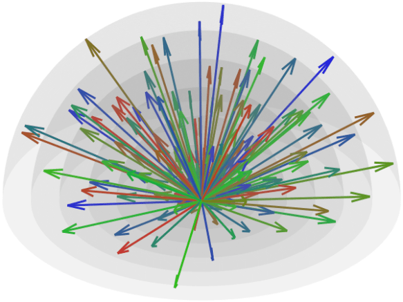
Since antipodal points are included in the cost function, all directions can, for visualization purposes, be represented in only one hemisphere. However, that is only for display; the vectors themselves have equal likelihood of being in one hemisphere or another, thus covering the whole surface of the sphere.
Order of arguments and of operations
The order the arguments are provided is not relevant. If the same argument is repeated, it is the last one that counts. Inside the program, the operations happen in the following order:
The options –new or –load are executed, thus either creating or loading a set of directions.
If a file in a format that does not include b-values was loaded, or if a new set of directions was just created, the option –bvalues is parsed, thus defining the b-values for each shell.
The option –reorder is executed if provided, thus optimally reordering the directions.
The option –removeb0 is executed if provided, thus removing directions that have been assigned a b-value = 0.
The option –addb0 is executed if provided, thus adding b-values = 0 and corresponding directions.
The option –save is executed if provided, thus saving the set of directions to a file in the specified format.
The option –plot is executed if provided, thus showing the directions (interactive mode) or saved to a file in the specified format (png, pdf, svg, eps, and various others supported by matplotlib).
Integration with your Python code
If you prefer not to use the function from the system shell and prefer instead to call it from your Python code, you can do that too. Place the file multishell.py where you can import it, then call the functions as needed. A simple example is:
import multishell as ms
import numpy as np

# Number of directions
K = 120

# Number of shells
S = 3

# b-values of each shell
blist = [1000, 2000, 3000]

# Distribute the number of directions across shells
Ks = ms.directions_per_shell(K, S, 'quadratically')

# Simultaneous optimization of all directions
vectors, shells = ms.simultaneous_optimization(Ks, alpha=0.75, maxiter=100)

# Optimally reorder the directions
vectors, shells, idx = ms.optimal_reordering(vectors, shells)

# b-values for each corresponding direction
bvalues = np.array(blist)[shells[:,0]][:,None]

# Save in FSL format
fileprefix = 'mydirs'
ms.write_fsl(fileprefix, vectors, bvalues)

# Plot
ms.plot_directions(vectors, bvalues=bvalues, colorby='acquisition', style='quiver', reproject=False)
Why a new implementation?
Two helpful implementations provided by Caruyer are available. One is a webtool that allows up to 5 shells and up to 500 directions be downloaded after estimation via incremental optimization, but it doesn’t allow specification of the weighting parameter , and only saves the directions in a tabular format that requires further manipulation before it can be used in the scanner. The other is a Python version that uses simultaneous optimization and provides finer control, but the shells are indexed differently from the webtool, and doesn’t include incremental optimization; it also doesn’t save directly in a format that can be used in common scanners. It allows plotting, but in my system figures appear incorrectly cropped. Conversion tools for Siemens and GE are available, but they require additional installation of packages for format changes that are relatively simple. For the webtool, there is always a risk that it may no longer be available in the future; as a concrete example, when the directions were downloaded for use in the Human Connectome Project (Sotiropoulos et al., 2013), it was located at a different address, hosted by the INRIA, now no longer accessible (broken link). Additionally, I could not understand Figure 2 in the original paper (compare with the figures above), and I had to implement it to understand what was going on. Finally, an all-in-one tool was much needed by our group as we plan on projects and need to find best use of scanner time. As this new implementation is helpful to us, it is hoped it will be helpful to you as well.
References
The most important reference is the original paper by Caruyer and colleagues, and which should be cited in case you use this reimplementation in your research:
Marek, Tervo-Clemmens et al. (2022) suggest that we need much larger sample sizes to investigate associations between common variability in brain structure or function and cognition or psychiatric symptomatology. That is true under the assumption that such associations, for complex, multifactorial cognitive or psychiatric phenotypes, and characteristics accessible with existing imaging methods, exist.
Unfortunately, the evidence provided seems to suggest the absence of such effects. In their article, Figure 2 shows overlap only for the distribution of effects, with peaks virtually at zero for three major studies, but no evidence for overlap of localized effects; Supplementary Figure 17 shows near-perfect correlation for average connectivity, but not for connectivity in relation to complex phenotypes. In Linke et al. (2021), we showed evidence that similar clinical presentations can emerge from disparate changes in brain connectivity, suggesting substantial diversity in the presentation of the underlying biological substrate, even for the same behavioral measurements.
It is possible that the aspects of human behavior that we consider relevant, and which guide our cognitive and clinical phenotyping, do not manifest themselves as measurable entities using available brain imaging methods. Merely increasing sample size with such phenotypes can only ensure statistically significant results for trivial, negligible effects, which may still fail to replicate. More investment on the development of techniques to probe yet unexplored aspects of the brain tissue, in vivo, and non-invasively, are more likely to be fruitful, without prejudice to the collection of large samples. The same holds for cognitive and clinical phenotypes, which need to be reliable, even if only indirectly mapped into aspects of human behavior.
Anderson M. Winkler, Daniel S. Pine, Julia O. Linke

 the repulsion force between particles represented by their positions (vectors)
  and
and  (Equation 3 in the paper):

 is the number of shells, and
  is the number of points (directions) on shell
  .
.
 is the total number of points across all shells.
 in the Cartesian space is provided in Equation 7 of the paper:
 are the axes directions in the Cartesian coordinate system, i.e.,
  , and where again the first term within brackets considers the repulsion forces of the particles themselves, whereas the second considers their antipodal representations.
 , as well as the corresponding term in the gradient function) as new charged particles, we avoid this problem: for the minimal case of two particles, the two directions will be orthogonal one to another, thus each one providing maximally unique information.
 ranges between 0 and 1 and controls how much we want to emphasize intra-shell repulsion forces (greater
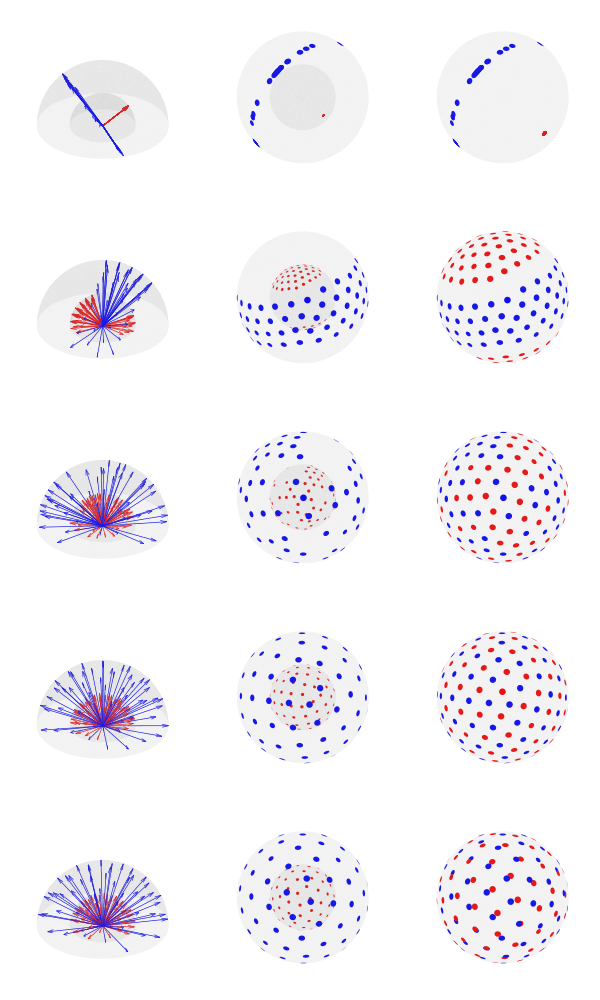
 of desired directions, the best solution can be found by starting with random vectors in the unit sphere, spread them across