
Preliminaries
Consider the common analysis of a neuroimaging experiment. At each voxel, vertex, face or edge (or any other imaging unit), we have a linear model expressed as:

where 


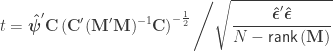
where the hat on 


When 
Permutation tests don’t depend on the same assumptions on which parametric tests are based. As some of these assumptions can be quite stringent in practice, permutation methods arguably should be preferred as a general framework for the statistical analysis of imaging data. At each permutation, a new statistic is computed and used to build its empirical distribution from which the p-values are obtained. In practice it’s not necessary to build the full distribution, and it suffices to increment a counter at each permutation. At the end, the counter is divided by the number of permutations to produce a p-value.
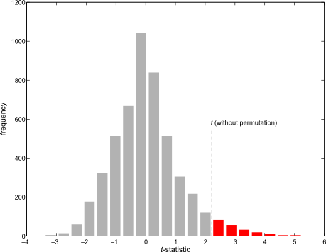
An example of a permutation distribution
Using permutation tests, correction for multiple testing using the family-wise error rate (fwer) is trivial: rather than build the permutation distribution at each voxel, a single distribution of the global maximum of the statistic across the image is constructed. Each permutation yields one maximum, that is used to build the distribution. Any dependence between the tests is implicitly captured, with not need to model it explicitly, nor to introduce even more assumptions, a problem that hinders methods such as the random field theory.
Exchangeability blocks
Permutation is allowed if it doesn’t affect the joint distribution of the error terms, i.e., if the errors are exchangeable. Some types of experiments may involve repeated measurements or other kinds of dependency, such that exchangeability cannot be guaranteed between all observations. However, various cases of structured dependency can still be accommodated if sets (blocks) of observations are shuffled as a whole, or if shuffling happens only within set (block). It is not necessary to know or to model the exact dependence structure between observations, which is captured implicitly as long as the blocks are defined correctly.
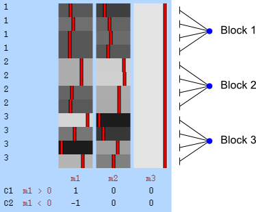
Permutation within block.
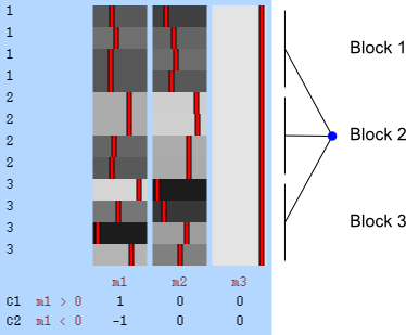
Permutation of blocks as a whole.
The two figures above are of designs constructed using the fsl software package. In fsl, within-block permutation is available in randomise with the option -e, used to supply a file with the definition of blocks. For whole-block permutation, in addition to the option -e, the option --permuteBlocks needs to be supplied.
The G-statistic
The presence of exchangeability blocks solves a problem, but creates another. Having blocks implies that observations may not be pooled together to produce a non-linear parameter estimate such as the variance. In other words: the mere presence of exchangeability blocks, either for shuffling within or as a whole, implies that the variances may not be the same across all observations, and a single estimate of this variance is likely to be inaccurate whenever the variances truly differ, or if the groups don’t have the same size. This also means that the F or t statistics may not behave as expected.
The solution is to use the block definitions and the permutation strategy is to define groups of observations that are known or assumed to have identical variances, and pool only the observations within group for variance estimation, i.e., to define variance groups (vgs).
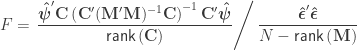
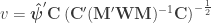
The F-statistic, however, doesn’t allow such multiple groups of variances, and we need to resort to another statistic. In Winkler et al. (2014) we propose:
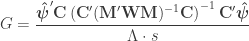
where 
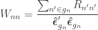
and where 


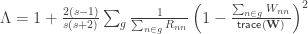
where 
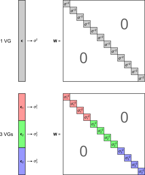
The W matrix used with the G statistic. It is constructed from the estimated variances of the error terms.
The matrix
When 

|
 |
|
|---|---|---|
| Homoscedastic errors, unrestricted exchangeability | Square of Student’s t | F-ratio |
| Homoscedastic within vg, restricted exchangeability | Square of Aspin-Welch |
Welch’s  |
In the absence of variance groups (i.e., all observations belong to the same vg), G and
Although not typically necessary if permutation methods are to be preferred, approximate parametric p-values for the G-statistic can be computed from an F-distribution with 

While the error rates are controlled adequately (a feature of permutation tests in general), the G-statistic offers excellent power when compared to the F-statistic, even when the assumptions of the latter are perfectly met. Moreover, by preserving pivotality, it is an adequate statistic to control of the error rate in the in the presence of multiple tests.
In this post, the focus is in using G for imaging data, but of course, it can be used for any dataset in which a linear model where variances cannot be assumed to be the same is used, i.e., when heteroscedasticity is or could be present.
Note that the G-statistic has nothing to do with the G-test. It is named as this for being a generalisation over various tests, including the commonly used t and F tests, as shown above.
Main reference
The core reference and results for the G-statistic have just been published in Neuroimage:
- Winkler AM, Ridgway GR, Webster MA, Smith SM, Nichols TE. Permutation inference for the general linear model. Neuroimage. 2014;92:381-397
Other references
The two other references cited, which are useful to understand the variance estimator and the parametric approximation are:
- Horn S, Horn R, Duncan D. Estimating heteroscedastic variances in linear models. J Am Stat Assoc. 1975;70(350):380–385.
- Welch B. On the comparison of several mean values: an alternative approach. Biometrika. 1951;38(3):330–336.
